Importing Modules and Installing Packages in Colab

Hello! In the previous lesson, you gave task-processing logic a name by writing functions. You can now reuse your own code. This lesson adds two ways to use code written elsewhere: import a module that Python already provides, and install a package into a Colab runtime before importing it. You’ll also arrange your notebook so those imports work again when Colab gives you a fresh runtime.

Allow about 35–40 minutes to read, watch the short video segments, and run the cells. You do not need a GPU for this lesson.

Import code that is already available

A module is a file of Python code containing names you can use, such as functions. Python supplies a collection of modules called the standard library. The math module, for example, provides ceil(), which rounds a number up to the next integer. It needs no installation.

In a Colab code cell, run:

import math

tasks = 11
tasks_per_group = 4
groups_needed = math.ceil(tasks / tasks_per_group)

print(groups_needed)  # 3

The division gives 2.75; processing all 11 tasks in groups of at most four takes three groups. In math.ceil(...), the dot says to find ceil inside the imported math module. This makes the origin of the function visible when you read the code.

You can use an imported function inside a function of your own:

import math

def groups_needed(task_count, group_size):
    """Return the number of groups needed for a task count."""
    return math.ceil(task_count / group_size)

print(groups_needed(11, 4))  # 3

This builds directly on the last lesson: your function defines when and why to calculate a result; the imported module supplies one part of the calculation.

There is another import form when you want a name directly available:

from math import ceil

print(ceil(11 / 4))  # 3

Both forms use the same function. For now, prefer import math when the module name helps make code clear. You will also encounter aliases, such as import math as m; the alias changes the name you type in the notebook, not the module itself.

Install a package into Colab

An import makes available code that the current Python environment can already find. An installation adds a package to that environment. Many AI libraries come preinstalled in Colab, but you should not assume every package—or a particular version—is present in every runtime.

Watch the first part of Google Colab - Installing Libraries! by Adrian Dolinay. The presenter uses a command prefixed with ! to inspect Colab’s installed libraries, then installs one that is missing. Focus on the distinction between the installation command and the subsequent Python import; you need not copy the video’s package or its error-handling code.

The Python packaging documentation gives the general rule behind the notebook commands. Read just the indicated portions; the other installation methods on that page are not needed today.

In Colab, use the notebook command %pip install for this lesson. It is a notebook command, not Python syntax. Colab also accepts shell commands prefixed with !, as the video shows; %pip is convenient because it installs into the environment associated with the current notebook kernel.

Try a small package that turns text into large printed letters. Put the installation in its own cell, above any cell that imports the package:

%pip install pyfiglet

Wait for that cell to finish. Then, in the next cell:

import pyfiglet

banner = pyfiglet.figlet_format("AI", font="small")
print(banner)

Here pyfiglet is both the package name used for installation and the module name used for import. That convenient match is not guaranteed for every package: an installation name and an import name can differ. The practical sequence is to install using the package’s installation name, then import using its documented Python name.

If you want to inspect what was installed, run this in another cell:

%pip show pyfiglet

It displays information such as the installed version. For work that needs repeatable results, a tested version can be specified in an installation command; today, the unpinned command keeps the first installation straightforward. Install packages you trust, because installed code runs in your environment.

Make the notebook usable with a fresh runtime

Your notebook holds the saved cells; the runtime is the temporary computer executing them. Saving the notebook preserves the installation command, not the package installation itself. If Colab replaces or discards the runtime, packages you added during that session may be gone. Likewise, imported names and variables must be created again by running their cells.

Watch only the beginning of the video’s later discussion. It demonstrates the problem after a fresh environment appears; you do not need its more elaborate approach to storing packages elsewhere.

For this lesson, the simplest reliable approach is to keep the setup steps near the top of the saved notebook, in this order:

1. Install any packages the runtime might not already have, such as %pip install pyfiglet.
2. Import the modules your code uses, such as import math and import pyfiglet.
3. Run cells that define functions and produce results.

Then a fresh runtime can run the notebook from top to bottom. If Colab says an installation requires a restart, follow that prompt and run the cells again afterward. Merely rerunning a later cell that says import pyfiglet will not replace a missing installation step.

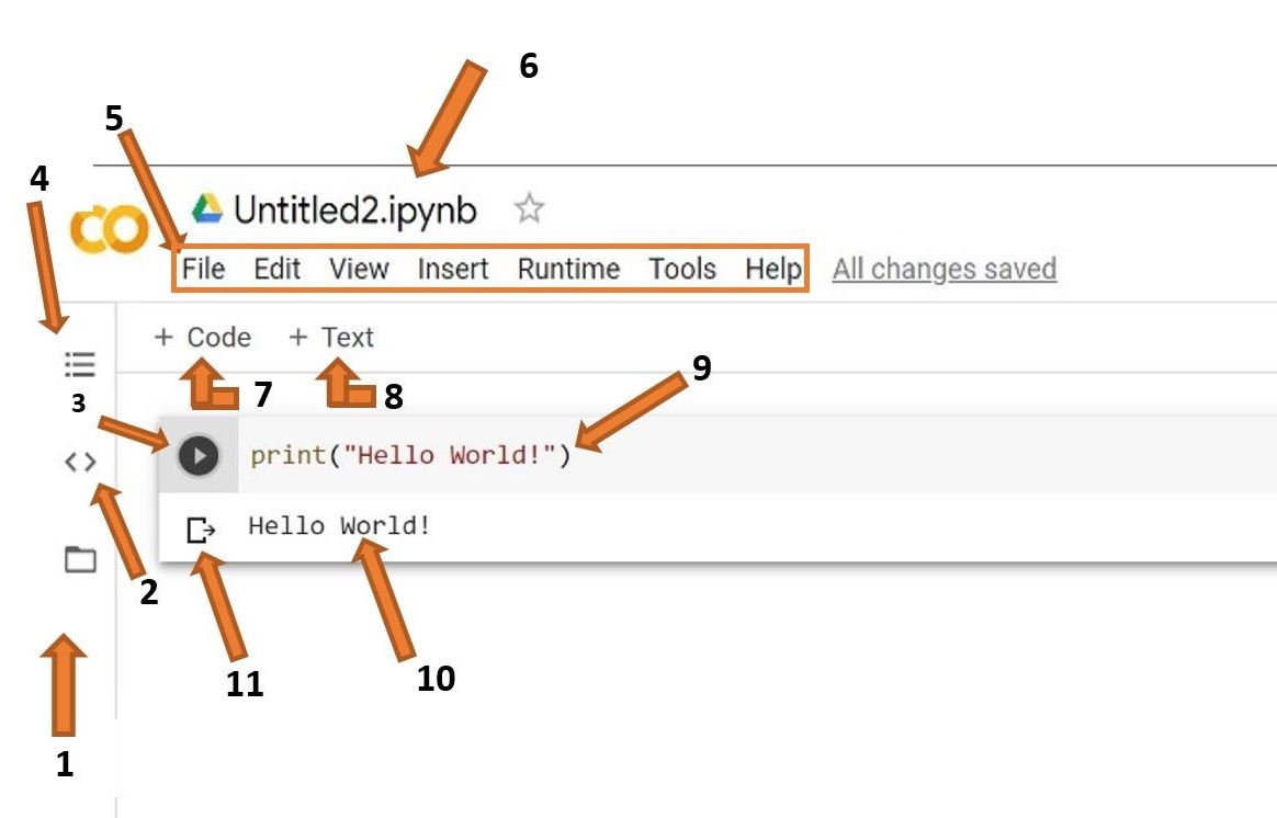
The labeled Colab interface below shows the + Code button for adding cells, the play button for running one, and the output area beneath a cell. Your interface may look slightly different, but these are the controls you need to put setup before use.

For a clean notebook, you could combine the imports in one cell after installation:

import math
import pyfiglet

print(f"Groups needed: {math.ceil(11 / 4)}")
print(pyfiglet.figlet_format("AI", font="small"))

Running cells out of order can make a notebook appear to work only because an earlier, now-hidden step already ran in the current runtime. Running from the top after a fresh runtime checks that the saved notebook contains everything it needs for this example.

Takeaway

Use import to access code available to your Python runtime; use %pip install in Colab to add a package that the runtime needs. Keep installation cells before imports, and remember that saved notebook cells persist even when their runtime’s added packages and variables do not. In the next lesson, you’ll use the errors Python displays—including those caused by missing names or modules—to find and correct problems in your code.