Gradients of MSE and Cross-Entropy Losses

Introduction

In our previous lesson, we established the softmax function as the essential tool for converting the raw, unbounded logits from a neural network's final layer into a valid probability distribution over multiple classes. We now have a vector of predicted probabilities, $\mathbf{p}$. The next logical step is to quantify how "wrong" these predictions are compared to the actual ground truth. This is the role of a loss function, also known as a cost or objective function.

This lesson focuses on deriving the gradients of the two most fundamental loss functions in neural networks: Mean Squared Error (MSE) for regression tasks and Cross-Entropy for classification. Our goal is not just to define these functions, but to compute their derivatives with respect to the network's final logits, $\mathbf{z}$. This specific gradient, $\frac{\partial \mathcal{L}}{\partial \mathbf{z}}$, is the linchpin of the entire training process. It represents the initial error signal that we will propagate backward through the network to update all its parameters—a process we will fully dissect in our next lesson on backpropagation.

Mean Squared Error (MSE) for Regression

Let's begin with the "Classical to Modern Bridge." In classical linear regression, where the goal is to predict a continuous value, the Mean Squared Error is the standard loss function. It measures the average of the squared differences between the predicted values and the actual values. This same principle applies directly to neural networks designed for regression tasks, such as predicting the price of a house or the trajectory of an object.

For a regression network, the output layer typically has a linear activation function (or no activation at all), meaning the output prediction ${\hat{y}}_k$ is simply the logit $z_k$. For a single prediction $\hat{y}$ and a single true label $y$, the loss is:

$${\mathcal{L}}_{MSE}=\frac{1}{2}(\hat{y}-y{)}^2$$

The factor of $\frac{1}{2}$ is a common convention that simplifies the derivative without changing the location of the minimum.

Now, consider a network with $K$ output neurons, predicting a vector of $K$ continuous values. The prediction vector is $\hat{\mathbf{y}}=\mathbf{z}$ and the true label vector is $\mathbf{y}$. The MSE loss is the sum of squared errors for each component:

$${\mathcal{L}}_{MSE}=\frac{1}{2}\sum _{k=1}^K({\hat{y}}_k-y_k{)}^2=\frac{1}{2}\sum _{k=1}^K(z_k-y_k{)}^2$$

Our task is to find the gradient of this loss with respect to the logit vector $\mathbf{z}$, which is ${\nabla }_{\mathbf{z}}\mathcal{L}$. To do this, we can compute the partial derivative with respect to an arbitrary logit $z_j$.

Question: When you take the partial derivative $\frac{\partial {\mathcal{L}}_{MSE}}{\partial z_j}$, which term in the summation ${\sum }_{k=1}^K(z_k-y_k{)}^2$ is the only one that does not evaluate to zero? Using this insight, what is the resulting partial derivative?

Answer

The derivative of a sum is the sum of the derivatives. When differentiating with respect to $z_j$, all terms $(z_k - y_k)^2$ where $k \neq j$ are treated as constants, and their derivatives are zero. The only term that survives is the one where $k=j$.

Applying the power rule and chain rule to this term gives:

$$\frac{\partial {\mathcal{L}}_{MSE}}{\partial z_j}=\frac{\partial }{\partial z_j}\left[\frac{1}{2}(z_j-y_j{)}^2\right]=\frac{1}{2}\cdot 2(z_j-y_j)\cdot \frac{\partial }{\partial z_j}(z_j-y_j)=z_j-y_j$$

This gives us a remarkably simple and intuitive result. The gradient of the MSE loss with respect to a single logit $z_j$ is simply the error for that output, $z_j-y_j$. Therefore, the gradient vector for all logits is:

$${\nabla }_{\mathbf{z}}{\mathcal{L}}_{MSE}=\mathbf{z}-\mathbf{y}=\hat{\mathbf{y}}-\mathbf{y}$$

The error signal that needs to be propagated backward is simply the vector of differences between our predictions and the true values.

The article below formally defines various loss functions and derives this exact gradient for linear regression, which is identical to our neural network regression case.

Cross-Entropy Loss for Classification

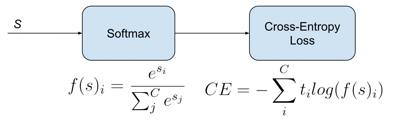
For classification tasks, where the network output is a probability distribution $\mathbf{p}=\text{softmax}(\mathbf{z})$, MSE is generally not the best choice. Instead, we use the cross-entropy loss. From an information theory perspective, this loss measures the dissimilarity between the predicted probability distribution $\mathbf{p}$ and the true distribution $\mathbf{y}$ (which is a one-hot vector).

The multi-class cross-entropy loss for a single training example is defined as:

$${\mathcal{L}}_{CE}=-\sum _{k=1}^K{y}_k\log (p_k)$$

Where $y_k$ is 1 for the true class and 0 otherwise, and $p_k$ is the softmax probability for class $k$.

Because $\mathbf{y}$ is one-hot, this sum simplifies dramatically. If the correct class is $c$, then $y_c=1$ and all other $y_k=0$, so the loss becomes:

$${\mathcal{L}}_{CE}=-\log (p_c)$$

To minimize this loss, the network must maximize $\log (p_c)$, which is equivalent to making the predicted probability of the correct class, $p_c$, as close to 1 as possible. This aligns perfectly with the goal of classification.

Deriving the Gradient of Cross-Entropy with Softmax

Our goal is to find the gradient $\frac{\partial {\mathcal{L}}_{CE}}{\partial z_j}$. This is more involved than the MSE case because the loss is a function of the probabilities $\mathbf{p}$, which are themselves a function of the logits $\mathbf{z}$.

Question: Given the functional composition $\mathcal{L}(\mathbf{p}(\mathbf{z}))$, what mathematical rule must we invoke to find the derivative of the loss $\mathcal{L}$ with respect to the logits $\mathbf{z}$?

Answer

We must use the **multivariable chain rule**. The influence of a single logit $z_j$ on the final loss $\mathcal{L}$ is channeled through *all* the probabilities $p_1, p_2, ..., p_K$, because a change in one logit affects all outputs of the softmax function.

The chain rule states:

$$\frac{\partial \mathcal{L}}{\partial z_j}=\sum _{i=1}^K\frac{\partial \mathcal{L}}{\partial p_i}\frac{\partial p_i}{\partial z_j}$$

This expression elegantly breaks our problem into two parts we already know how to solve:

1. $\frac{\partial \mathcal{L}}{\partial p_i}$: The derivative of the cross-entropy loss with respect to an output probability.
2. $\frac{\partial p_i}{\partial z_j}$: The derivative of the softmax function, which we derived in the last lesson. This is an element of the softmax Jacobian matrix.

Let's compute these parts and assemble the result.

Part 1: Derivative of Loss w.r.t. Probability
For $\mathcal{L}=-{\sum }_k{y}_k\log (p_k)$, the derivative with respect to a single probability $p_i$ is:

$$\frac{\partial \mathcal{L}}{\partial p_i}=-\frac{y_i}{p_i}$$

Part 2: Derivative of Softmax (from last lesson)
We have two cases for $\frac{\partial p_i}{\partial z_j}$:

• Case $i=j$: $\frac{\partial p_i}{\partial z_i}=p_i(1-p_i)$
• Case $i\ne j$: $\frac{\partial p_i}{\partial z_j}=-p_i{p}_j$

Part 3: Assembling with the Chain Rule
We expand the sum from the chain rule, splitting it into the $i=j$ term and the sum over all $i\ne j$ terms:

$$\frac{\partial \mathcal{L}}{\partial z_j}=\underset{i=j\text{ term}}{\underbrace{\left(\frac{\partial \mathcal{L}}{\partial p_j}\frac{\partial p_j}{\partial z_j}\right)}}+\underset{i\ne j\text{ terms}}{\underbrace{\sum _{i\ne j}\left(\frac{\partial \mathcal{L}}{\partial p_i}\frac{\partial p_i}{\partial z_j}\right)}}$$

Now, substitute the derivatives we found:

$$\frac{\partial \mathcal{L}}{\partial z_j}=\left(-\frac{y_j}{p_j}\right)\cdot \left(p_j(1-p_j)\right)+\sum _{i\ne j}\left(-\frac{y_i}{p_i}\right)\cdot \left(-p_i{p}_j\right)$$

Let's simplify this expression step-by-step:

1. Cancel terms in each part: $$\frac{\partial \mathcal{L}}{\partial z_j}=-y_j(1-p_j)+\sum _{i\ne j}{y}_i{p}_j$$
2. Distribute $-y_j$ and factor $p_j$ out of the sum: $$\frac{\partial \mathcal{L}}{\partial z_j}=-y_j+y_j{p}_j+p_j\sum _{i\ne j}{y}_i$$
3. Factor out $p_j$ from the last two terms: $$\frac{\partial \mathcal{L}}{\partial z_j}=-y_j+p_j\left(y_j+\sum _{i\ne j}{y}_i\right)$$
4. Recognize that since $\mathbf{y}$ is one-hot, the term in the parenthesis is simply the sum of all elements of $\mathbf{y}$, which is ${\sum }_{k=1}^K{y}_k=1$. $$\frac{\partial \mathcal{L}}{\partial z_j}=-y_j+p_j(1)=p_j-y_j$$

This yields an astonishingly simple and elegant result. The gradient of the combined softmax and cross-entropy loss with respect to a logit $z_j$ is simply the difference between the predicted probability $p_j$ and the true label $y_j$. The full gradient vector is:

$${\nabla }_{\mathbf{z}}{\mathcal{L}}_{CE}=\mathbf{p}-\mathbf{y}$$

The following video provides a complete, step-by-step walkthrough of this exact derivation. Watching it will help solidify your understanding of each algebraic manipulation.

A Unified View: Prediction - Label

Let's take a step back and compare the gradients we've derived.

• Regression with MSE: ${\nabla }_{\mathbf{z}}\mathcal{L}=\mathbf{z}-\mathbf{y}$
• Classification with Softmax + Cross-Entropy: ${\nabla }_{\mathbf{z}}\mathcal{L}=\mathbf{p}-\mathbf{y}$

In both cases, the gradient has the same intuitive structure: $\text{prediction}-\text{label}$. For regression, the prediction is the logit vector $\mathbf{z}$. For classification, the prediction is the probability vector $\mathbf{p}$. This is a powerful and unifying concept in the design of neural networks and loss functions. The error signal that initiates backpropagation is a direct measure of how wrong the network's prediction was.

Conclusion

In this lesson, we have derived the crucial starting gradients for the backpropagation algorithm. We have seen how to measure the error of a neural network's output and, more importantly, how to calculate the sensitivity of that error with respect to the pre-activation logits.

Key Takeaways:

• Loss Functions Quantify Error: MSE is the standard for regression, while Cross-Entropy is the standard for classification.
• Gradient for MSE: For a regression network with linear outputs, the gradient of the MSE loss with respect to the logits is simply $\mathbf{z}-\mathbf{y}$.
• Gradient for Cross-Entropy: The combination of a Softmax output layer and a Cross-Entropy loss function results in a beautifully simple gradient with respect to the logits: $\mathbf{p}-\mathbf{y}$.
• Unified Pattern: Both scenarios result in a gradient of the form prediction - label, providing a powerful and intuitive starting point for training.

Preview of the Next Lesson:

With the "head" of the gradient, $\frac{\partial \mathcal{L}}{\partial \mathbf{z}}$, now fully derived, we are ready to tackle the main event: deriving the full backpropagation algorithm. We will apply the chain rule recursively to propagate this initial error signal backward through the network's layers, computing the gradients with respect to every weight and bias, $\frac{\partial \mathcal{L}}{\partial \mathbf{W}}$ and $\frac{\partial \mathcal{L}}{\partial \mathbf{b}}$. This will give us everything we need to finally start training a neural network.