Forward Pass in Multi-Layer Networks

Introduction

In our previous lesson, we assembled the architectural blueprint of a feedforward neural network, understanding it as a composite function built from layers. Each layer performs an affine transformation followed by a non-linear activation. We established what a network is. Now, we will explore how it operates.

This lesson focuses on the forward pass, the fundamental process of taking an input and propagating it through the network's layers to produce a final prediction. This mechanism is not only how a trained model performs inference on new data but also constitutes the first of two critical stages in the training cycle. For you, with an eye towards performance and low-level engineering, understanding this data flow is paramount, as it's the core computational workload that systems like GPUs are designed to accelerate.

The Flow of Information

At its heart, the forward pass is a sequential chain of computations. The output of one layer becomes the input for the next. Let's visualize this with a simple three-layer network.

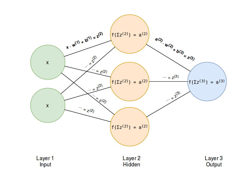
This diagram illustrates the entire process. Let's break down the notation, aligning it with the formalism from our last lesson where the superscript [l] denotes the $l$-th layer:

1. Input Layer (Layer 1): We start with the input vector, denoted as $\mathbf{x}$. In the diagram, this is "Layer 1".

2. Hidden Layer (Layer 2):

   • An affine transformation is applied to the input $\mathbf{x}$. The diagram shows this as x . w(1) + b(1) = z(2). In our notation, this is ${\mathbf{z}}^{[2]}={\mathbf{W}}^{[2]}\mathbf{x}+{\mathbf{b}}^{[2]}$. The matrix ${\mathbf{W}}^{[2]}$ contains the weights connecting the input to the hidden layer, and ${\mathbf{b}}^{[2]}$ is the bias vector for the hidden layer.
   • A non-linear activation function, $f$, is applied element-wise to ${\mathbf{z}}^{[2]}$ to produce the hidden layer's activations, ${\mathbf{a}}^{[2]}$. The diagram labels this f(Σz(2)) = a(2). The summation symbol here is slightly confusing; it's more accurate to think of this as the function $f$ being applied to each element of the vector ${\mathbf{z}}^{[2]}$ individually.

3. Output Layer (Layer 3):

   • The process repeats. The activations from the hidden layer, ${\mathbf{a}}^{[2]}$, are now the input to the output layer. The affine transformation is ${\mathbf{z}}^{[3]}={\mathbf{W}}^{[3]}{\mathbf{a}}^{[2]}+{\mathbf{b}}^{[3]}$.
   • A final activation function is applied to get the network's prediction, $\hat{\mathbf{y}}={\mathbf{a}}^{[3]}=f({\mathbf{z}}^{[3]})$.

This flow from input to output, without any loops, is why these are called feedforward networks.

The Forward Pass and the Computation Graph

In our last lesson, we introduced the concept of a computation graph. The forward pass is nothing more than evaluating this graph from the input nodes to the final output node. Each node performs a simple, local computation, and the directed edges dictate the flow of data.

This perspective is crucial for implementing complex models. Instead of a monolithic equation, we have a modular structure of operations. The following video offers a clear, step-by-step walkthrough of a forward pass on a simple computation graph.

The video demonstrates a key principle: the forward pass populates the graph with concrete numerical values based on a specific input. The structure of the graph itself is defined by our network architecture, but the values within it are determined by the input data and the current parameters (weights and biases).

From Single Vectors to Batches: A Performance Perspective

So far, we have considered processing a single input vector $\mathbf{x}$. From a systems programming viewpoint, this is inefficient. The overhead of launching a computation for one small vector is high. To leverage the parallel processing power of modern hardware, especially GPUs, we process a batch of inputs simultaneously.

Instead of an input vector $\mathbf{x}\in {\mathbb{R}}^{d_{in}}$ (where $d_{in}$ is the number of features), we work with an input matrix $\mathbf{X}\in {\mathbb{R}}^{n\times d_{in}}$, where $n$ is the batch size.

This changes our layer computation from matrix-vector products to matrix-matrix products. For a layer $l$ with $d_{out}$ neurons, taking input activations ${\mathbf{A}}^{[l-1]}\in {\mathbb{R}}^{n\times d_{in}}$:

1. Affine Transformation: ${\mathbf{Z}}^{[l]}={\mathbf{A}}^{[l-1]}{\mathbf{W}}^{[l]}+{\mathbf{b}}^{[l]}$

   • ${\mathbf{W}}^{[l]}$ is the weight matrix of size $d_{in}\times d_{out}$.
   • The product ${\mathbf{A}}^{[l-1]}{\mathbf{W}}^{[l]}$ results in a matrix of size $n\times d_{out}$.
   • ${\mathbf{b}}^{[l]}$ is the bias vector of size $1\times d_{out}$. Through an operation called broadcasting, this bias vector is added to every row of the preceding product matrix. This avoids an explicit loop and is highly optimized in numerical computing libraries.

2. Non-linear Activation: ${\mathbf{A}}^{[l]}=g({\mathbf{Z}}^{[l]})$

   • The activation function $g$ is applied element-wise to the entire matrix ${\mathbf{Z}}^{[l]}$, producing the final activation matrix ${\mathbf{A}}^{[l]}\in {\mathbb{R}}^{n\times d_{out}}$.

This batched approach replaces many small operations with a few large matrix operations, which is exactly what GPUs are built for. The following article details this process, including a clever technique called the "bias trick" that formally incorporates the bias into the weight matrix.

A Concrete Example

Let's solidify this with a numerical example. Consider a 2-layer network: a hidden layer with 2 neurons (using ReLU) and an output layer with 1 neuron (using Sigmoid).

• Input: $\mathbf{x}=[2.0,3.0{]}^T$
• Hidden Layer (l=1):
  • Weights: ${\mathbf{W}}^{[1]}=\left(\begin{array}{cc}0.2& -0.5\\ 0.4& 0.1\end{array}\right)$ (Note: I've transposed the matrix from the thought block to match the $\mathbf{Wx}$ convention here, where columns correspond to input features)
  • Bias: ${\mathbf{b}}^{[1]}=[0.1,-0.2{]}^T$
• Output Layer (l=2):
  • Weights: ${\mathbf{W}}^{[2]}=[0.7,-0.3]$
  • Bias: ${\mathbf{b}}^{[2]}=[0.5]$

Step 1: Forward Pass through Hidden Layer

First, the affine transformation:

Next, apply the ReLU activation function element-wise:

The output of the hidden layer is $[0,0.9{]}^T$. Notice how the ReLU activation "turned off" the first neuron.

Step 2: Forward Pass through Output Layer

The input is now ${\mathbf{a}}^{[1]}$. We perform the next affine transformation:

Finally, apply the Sigmoid activation to get the prediction:

The final prediction of our network for the input $[2.0,3.0{]}^T$ is approximately 0.557.

Implementation From First Principles

For someone interested in low-level engineering, seeing the code that executes this process is illuminating. The following C++ code implements the forward pass for a single feedforward node.

Conclusion

In this lesson, we have demystified the forward pass, tracing the path of data from input to prediction. We've seen how a sequence of simple, local computations—affine transformations and non-linear activations—combine to produce the network's output.

Key Takeaways:

• The forward pass is a sequential evaluation of the network's layers to compute a prediction $\hat{\mathbf{y}}$ from an input $\mathbf{x}$.
• From a graph perspective, it is a left-to-right traversal of the computation graph.
• For performance, inputs are processed in batches, transforming the computation into a series of large matrix-matrix multiplications.
• This process is the core of inference and the first half of the training loop.

Preview of the Next Lesson:

Our network has made a prediction, $\hat{\mathbf{y}}$. But is it a good prediction? To train the network, we must quantify its error. In the next lesson, we will introduce loss functions, which measure the discrepancy between the predicted output ($\hat{\mathbf{y}}$) and the true target ($\mathbf{y}$). We will then derive the gradient of the loss with respect to the network's final output, which is the crucial first step of the backward pass, or backpropagation.