Affine Transformations in 3D Using Homogeneous Coordinates

Welcome. This course begins with the mathematical and PyTorch foundations you will use to work with 3D data, then builds toward point clouds, meshes, equivariant models, and research practice. Today’s distinction is small but consequential: a point is a location, while a displacement vector describes an offset between locations. You will learn to transform both with the same $4\times 4$ matrix without accidentally translating a displacement.

This lesson should take about 40 minutes, including the video, reading, and code.

Why add a fourth coordinate?

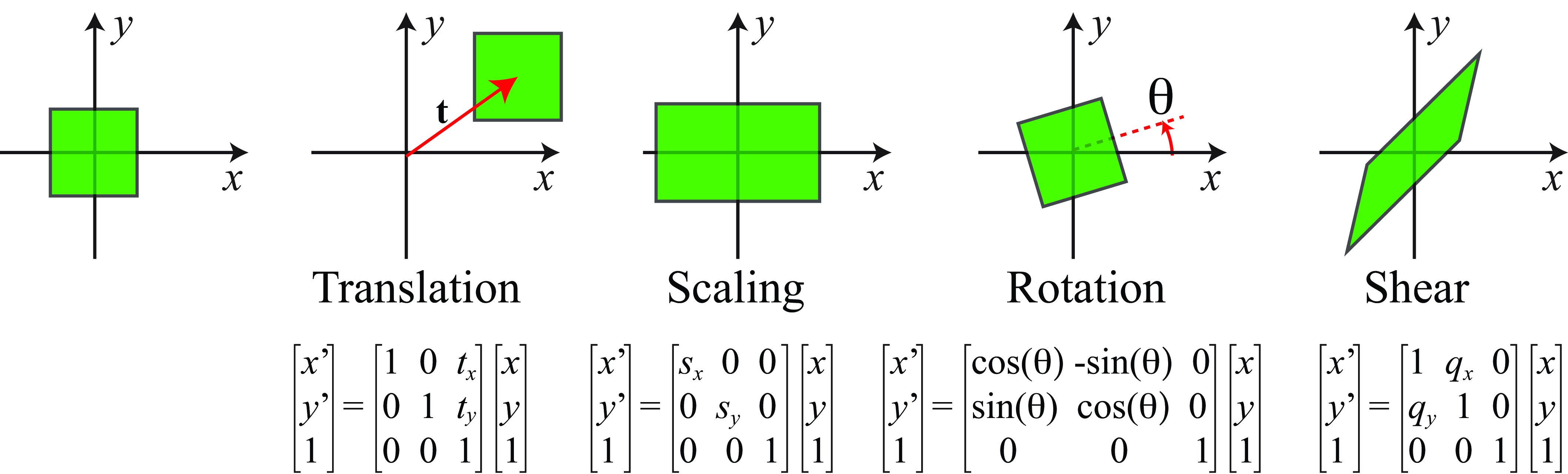
A linear transformation of 3D coordinates has the form ${\mathbf{p}}^{\prime }=A\mathbf{p}$, where $A$ is a $3\times 3$ matrix. It can rotate, scale, reflect, or shear, but it cannot move the origin: $A0=0$. To include a translation $\mathbf{t}$, we need an affine transformation:

The image shows the 2D version. Notice that translation occupies a separate column of each $3\times 3$ matrix; the same arrangement becomes a $4\times 4$ matrix in 3D.

Watch only the opening of the following video. Its game-engine setting is incidental; focus on why the extra coordinate makes translation part of matrix multiplication.

For a 3D point, append $1$; for now, think of it as a switch that allows the translation column to contribute:

The bottom row keeps the last coordinate equal to $1$. Here $A$ can be any $3\times 3$ linear transformation; it need not be a rotation. For the affine matrices in this lesson, there is no need to divide the resulting coordinates by the last entry. That division becomes relevant later for perspective projection.

Points move; displacements do not translate

Suppose $\mathbf{p}$ and $\mathbf{q}$ are two locations. Their difference $\mathbf{v}=\mathbf{q}-\mathbf{p}$ is a displacement. If both locations undergo the same affine transformation, their new difference is

Translation cancels. The displacement may still rotate, scale, or shear because $A$ acts on it.

Homogeneous coordinates encode this distinction by appending $0$ to a displacement:

The translation column is multiplied by zero. Do not divide a displacement’s coordinates by its last entry: it is zero. Instead, read the first three entries as the transformed displacement.

This gives a useful consistency rule. A point plus a displacement is another point, and subtracting two points gives a displacement. Their homogeneous last entries behave accordingly: $1+0=1$ and $1-1=0$. In point-cloud work, this rule prevents a common error: if you reposition an entire cloud, the offsets between its points must not acquire the cloud’s translation.

Compose transformations in the order you intend

Homogeneous matrices are useful because several affine operations can be combined into one matrix. With the column-vector convention used here, the rightmost matrix acts first. Read the worked example in LearnOpenGL before following the 3D calculation below.

Consider a scale by $2$ in the $x$-direction, followed by a $90^{\circ }$ rotation about the $z$-axis, followed by translation by $\mathbf{t}=(3,-1,2{)}^{\top }$. With column vectors, the combined matrix is $T_{\mathrm{translate}}{T}_{\mathrm{rotate}}{T}_{\mathrm{scale}}$. Its upper-left block is

For $\mathbf{p}=(1,2,0{)}^{\top }$, the transformed point is

But the displacement $\mathbf{v}=(1,2,0{)}^{\top }$, despite having the same three numbers, becomes $(-2,2,0{)}^{\top }$. Its meaning—and therefore its fourth coordinate—is different.

Order matters for points. If you translated before applying $A$, the result would be $A(\mathbf{p}+\mathbf{t})=A\mathbf{p}+A\mathbf{t}$, not $A\mathbf{p}+\mathbf{t}$. The earlier translation would itself be rotated and scaled.

An affine transformation preserves straight lines and parallelism, but an arbitrary $A$ need not preserve lengths or angles. The scale in this example changes some distances; a rotation followed by translation, without scaling or shear, would preserve them.

When the matrix describes a change of coordinates

So far, we have treated $T$ as an operation that moves points. The same matrix form can also describe a different task: expressing an unchanged physical point in a different coordinate frame. The arithmetic looks identical, so labels matter.

Suppose frame $B$ has its origin at $\mathbf{o}$ in world frame $W$, and its three basis vectors, expressed in world coordinates, form the columns of $B$. Then

For the point, ${\mathbf{p}}_W=B{\mathbf{p}}_B+\mathbf{o}$. For the displacement, ${\mathbf{v}}_W=B{\mathbf{v}}_B$: the position of frame $B$’s origin is irrelevant to an offset. If $F_{WB}$ is invertible, its inverse converts world coordinates back to frame $B$ coordinates:

For example, let $B$’s axes be rotated $90^{\circ }$ about the world $z$-axis, and let its origin be $\mathbf{o}=(3,-1,2{)}^{\top }$. The local point ${\mathbf{p}}_B=(1,0,0{)}^{\top }$ is the world point ${\mathbf{p}}_W=(3,0,2{)}^{\top }$. A local displacement ${\mathbf{v}}_B=(1,0,0{)}^{\top }$, however, is the world displacement ${\mathbf{v}}_W=(0,1,0{)}^{\top }$.

A matrix that moves a point in a fixed frame and one that changes the coordinates used to describe that point can have the same numerical entries. Before multiplying, state what the input coordinates are and what the output coordinates mean. This habit will be especially important when you encounter camera frames.

Apply and check the rule in PyTorch

The following small batch implements the scale–rotation–translation example. Rows store points, so the code transposes the batch while applying the column-vector matrix convention established above.

import torch

dtype = torch.float64

scale = torch.eye(4, dtype=dtype)
scale[:3, :3] = torch.diag(torch.tensor([2., 1., 1.], dtype=dtype))

rotate = torch.eye(4, dtype=dtype)
rotate[:2, :2] = torch.tensor([[0., -1.], [1., 0.]], dtype=dtype)

translate = torch.eye(4, dtype=dtype)
translate[:3, 3] = torch.tensor([3., -1., 2.], dtype=dtype)

T = translate @ rotate @ scale  # scale first, translate last

def transform_rows(x, last_coordinate):
    w = torch.full((x.shape[0], 1), last_coordinate, dtype=x.dtype)
    x_h = torch.cat((x, w), dim=1)
    return (T @ x_h.T).T[:, :3]

points = torch.tensor([[1., 2., 0.], [2., 4., 0.]], dtype=dtype)
offset = points[1:] - points[:1]

new_points = transform_rows(points, 1.)
new_offset = transform_rows(offset, 0.)

print(new_points)  # [[ 1., 1., 2.], [-1., 3., 2.]]
print(new_offset)  # [[-2., 2., 0.]]

assert torch.allclose(new_points[1:] - new_points[:1], new_offset)

The assertion checks a geometric fact, not just a pair of expected numbers: transforming the difference between points must agree with taking the difference after transforming the points. It would fail if you appended $1$ to the offset and inadvertently translated it. The matrix used here is invertible, so torch.linalg.inv(T) can also undo its effect on points; a zero scaling factor would make that impossible.

You now have the core rule: use a $4\times 4$ affine matrix with a trailing $1$ for a point and $0$ for a displacement. The $3\times 3$ block acts on both; the translation column acts only on points. Keep track of multiplication order and coordinate-frame labels, because correct arithmetic with the wrong interpretation still produces the wrong geometry.

Next, you will use PyTorch to compute batched pairwise distances between points in a cloud—an operation whose behavior under translation and rotation you can now reason about.