Recommended resources
The freely available resources this lesson will direct you to.
Welcome back. In the previous lesson, you used eigenvectors to identify directions associated with a matrix. Here the object is a scalar field: a function that assigns one number to each point in space. Its gradient tells you how that number changes when you move in different spatial directions.
You will compute a 3D gradient by hand using the chain rule, then check it with PyTorch autograd. Allow about 40 minutes for the video, reading, derivation, and code.
From a scalar value to a spatial direction
A scalar field in three dimensions is a function . Temperature is one example: a position has one temperature value . A model that assigns a numerical score to each 3D position is another.
The gradient collects the field’s three partial derivatives into a vector:
To compute the first component, vary while holding and fixed; do the analogous calculation for the other components. If is a unit direction, the rate of change per unit distance in that direction is . Where the gradient is nonzero, it points in the direction of greatest increase, and its length is that greatest rate.
Gradient of a scalar field | Multivariable Calculus | Khan Academy
Watch Gradient of a scalar field from Khan Academy for an example that starts with a value at every 3D position and computes a gradient at those positions.
Watch the scalar field for the distinction between a scalar value and a gradient vector. Then watch the calculation, focusing on why the other two coordinates are held fixed for each partial derivative and where the chain rule enters.
One visualization caution is useful for 3D work. A surface drawn as height represents a field with two spatial inputs; the height is its output. A field instead takes all three spatial coordinates as inputs. We can still use the height picture to understand how a gradient relates to movement through a field.
Use the chain rule inside the field—and along a path
Suppose a height field is , and a path across its domain is . The height experienced along the path is . Although has two spatial inputs, has one time input.
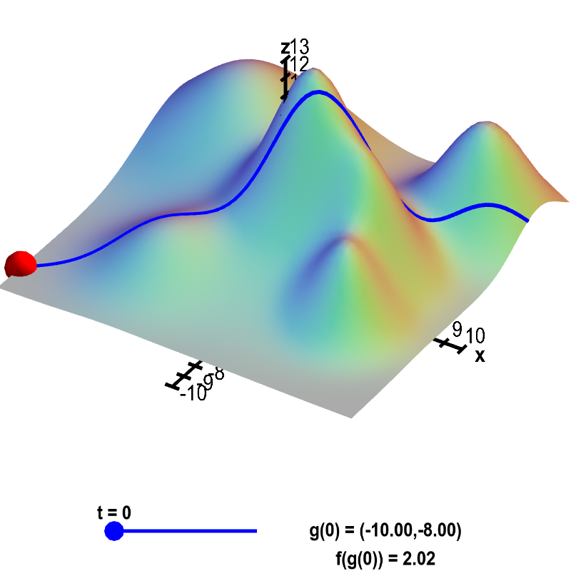
Introduction to the multivariable chain rule
Read Math Insight’s Introduction to the multivariable chain rule to connect spatial partial derivatives with the rate of change along a moving path.
In “The chain rule in two dimensions,” begin where the text redefines the mountain range as a two-variable function. Read the path example through the component-wise chain rule, ending at the observation that the one-variable rule has been applied twice. Focus on where the partial derivatives are evaluated and why both coordinates contribute to the rate of change.
For a 3D path , the same idea gives
This is a scalar rate along one chosen path, not the full gradient. The gradient supplies the spatial rates; the path velocity specifies how much you move in each direction. Notice also that the gradient is evaluated at the current position , not at the time .
Now apply the chain rule inside a field. Let be a fixed center, and define
The field is largest at and decreases with squared distance from it. Treat as the composition of and the one-variable function . Since , the chain rule gives
Holding the other coordinates fixed in turn yields
At , the squared distance is , so
That sign makes geometric sense: from , moving toward the center means moving in the negative -direction. At the center itself the gradient is zero. The field has a maximum there, but no single direction of increase at that point.
Verify the spatial gradient with autograd
PyTorch can differentiate the operations used to construct the field. Set requires_grad=True on the spatial input before evaluating the field; otherwise autograd will not track derivatives with respect to its coordinates.
import torch

center = torch.tensor([1.0, -1.0, 2.0], dtype=torch.float64)

def field(coords):
    squared_distance = ((coords - center) ** 2).sum(dim=-1)
    return 10.0 * torch.exp(-squared_distance)

p = torch.tensor(
    [2.0, -1.0, 2.0],
    dtype=torch.float64,
    requires_grad=True,
)

value = field(p)
grad_autograd = torch.autograd.grad(value, p)[0]
grad_analytic = -2.0 * (p - center) * value

print("field value:", value.item())
print("autograd gradient:", grad_autograd)
print("analytic gradient:", grad_analytic)

torch.testing.assert_close(
    grad_autograd, grad_analytic, rtol=1e-12, atol=1e-12
)
Here value is a scalar and grad_autograd has shape (3,): one derivative for each coordinate of p. The analytic expression is the same formula derived above, written using the already-computed value . Using float64 and an explicit tolerance makes the numerical comparison clear.
The field function also accepts an array of 3D points. For independently evaluated points, summing their scalar outputs lets autograd return one gradient per input point:
points = torch.tensor(
    [[2.0, -1.0, 2.0],
     [1.0,  0.0, 2.0],
     [1.0, -1.0, 2.0]],
    dtype=torch.float64,
    requires_grad=True,
)

values = field(points)                         # shape: (3,)
grads = torch.autograd.grad(values.sum(), points)[0]
expected = -2.0 * (points - center) * values[:, None]

print(grads)                                   # shape: (3, 3)
torch.testing.assert_close(grads, expected, rtol=1e-12, atol=1e-12)
The sum is needed because values is not a single scalar. In this example, each output depends only on its corresponding input row, so the gradient of the sum contains the three individual spatial gradients. That independence is an assumption of this calculation, not a property of every batched model.
Check what happens along a path
Finally, distinguish differentiation with respect to position from differentiation with respect to time. Consider
At , the path is at , with velocity . The path moves in both and , but at only the -component contributes to the instantaneous change in this field:
If you ran the first code block, you can compare this dot product with a second autograd calculation:
t = torch.tensor(0.0, dtype=torch.float64, requires_grad=True)

position = torch.stack((2.0 + t, -1.0 + t, 2.0 + 0.0 * t))
rate_autograd = torch.autograd.grad(field(position), t)[0]

velocity = torch.tensor([1.0, 1.0, 0.0], dtype=torch.float64)
rate_chain_rule = grad_autograd @ velocity

print("rate from autograd:", rate_autograd.item())
print("rate from chain rule:", rate_chain_rule.item())
torch.testing.assert_close(
    rate_autograd, rate_chain_rule, rtol=1e-12, atol=1e-12
)
The two autograd calls answer different questions. Differentiating with respect to p returns a 3D spatial gradient; differentiating with respect to t returns a single rate along the path. The chain rule connects them.
Takeaways
A scalar field assigns a number to each spatial position, while its gradient collects the partial derivatives into a vector. For a composed field, differentiate the outer function and each inner spatial expression; evaluate the resulting gradient at the point of interest. PyTorch autograd can verify the calculation, provided the spatial input is tracked and you check the output’s shape as well as its values.
Next, you will use the closely related Jacobian to describe how an entire coordinate transformation—not just a scalar field—changes near a point.