Recommended resources
The freely available resources this lesson will direct you to.
Hello! In the previous lesson, you calculated revenue for four storefront lines and practiced writing formulas that remain correct when copied. Now the question changes: how much revenue came from a particular platform or region, and how many lines produced it?
This lesson takes about 40 minutes, with most of that time spent building and checking a small Excel summary. You’ll use conditional aggregation functions to calculate totals, counts, and averages—skills you’ll use repeatedly when answering Data Analyst business questions.
A summary begins with a condition
Your earlier formula calculated revenue for each line. A conditional summary looks across many lines and includes only those that meet a rule. For example, “Shopify revenue in the US” requires a row to satisfy both conditions before its revenue contributes to the total.
Watch the first part of Leila Gharani’s How to Use SUMIFS, COUNTIFS and AVERAGEIFS in Excel (Multiple Criteria). Notice especially where the revenue range appears in SUMIF versus SUMIFS.
How to Use SUMIFS, COUNTIFS and AVERAGEIFS in Excel (Multiple Criteria)
Leila Gharani demonstrates a one-condition revenue total and then adds further conditions. Watch to understand the argument order before writing your own formulas.
Watch one condition for SUMIF, then multiple conditions for SUMIFS. As each formula is built, identify the column being summarized and the column tested by each condition.
Here is the key distinction:
| Question | Function | Argument pattern |
|---|---|---|
| Total revenue for one platform | SUMIF |
criteria range, criterion, sum range |
| Total revenue for one platform and region | SUMIFS |
sum range, criteria range, criterion, criteria range, criterion |
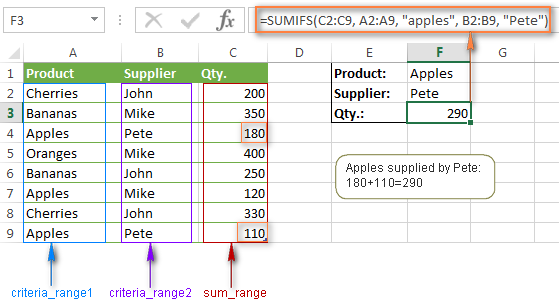
In SUMIFS, each criteria range–criterion pair tests the same set of rows. The function sums a row’s value only when all its conditions match. The image below illustrates this with apples supplied by Pete: the two qualifying quantities are 180 and 110, so the result is 290.
Build a storefront summary sheet
Add a new worksheet named ConditionalLab to the workbook you used previously. Keep StorefrontLines and ReferenceLab unchanged. This new dataset retains the first four line revenues from your earlier work and adds four lines so that platform and region comparisons are meaningful.
Enter these headers in A1:F1: LineID, Platform, Region, Units, UnitPrice, Revenue. Then enter the following data in A2:E9, leaving Revenue empty for now.
| LineID | Platform | Region | Units | UnitPrice |
|---|---|---|---|---|
| L1 | Shopify | US | 2 | 20 |
| L2 | Shopify | UK | 1 | 10 |
| L3 | Webflow | US | 1 | 20 |
| L4 | Unbounce | UK | 3 | 10 |
| L5 | Shopify | US | 3 | 10 |
| L6 | Shopify | UK | 2 | 25 |
| L7 | Webflow | UK | 3 | 5 |
| L8 | Unbounce | US | 5 | 5 |
Select A1:F9, press Ctrl+T, confirm My table has headers, and name the table SalesLines on the Table Design tab. In F2, enter:
=[@Units]*[@UnitPrice]
Excel should fill the formula down the table. Check that the eight revenues are 40, 10, 20, 30, 30, 50, 15, 25. Each row represents one product line, not necessarily one order or one customer. That distinction will matter when you interpret counts and averages.
Set up the summary area beside the table:
H3:Platform;I3:ShopifyH4:Region;I4:USH5:Minimum revenue;I5:25H7:Metric;I7:Result
The cells in column I are editable criteria. The dollar signs in formulas below keep those criteria references fixed if you later move or copy a formula, just as you practiced last lesson.
Calculate totals with one and two conditions
First, establish a number against which to check your summaries. Put All revenue in H8 and this formula in I8:
=SUM(SalesLines[Revenue])
You should get 220. The notation SalesLines[Revenue] refers to the table’s Revenue column. Unlike a fixed range such as F2:F9, it can include new rows added to the table.
Put Shopify revenue in H9. In I9, calculate the total for the platform selected in I3:
=SUMIF(SalesLines[Platform],$I$3,SalesLines[Revenue])
The result is 130. Read the formula in its argument order: look in the Platform column, match the value in I3, and sum Revenue for those rows.
Now put Shopify US revenue in H10 and enter:
=SUMIFS(SalesLines[Revenue],SalesLines[Platform],$I$3,SalesLines[Region],$I$4)
The result is 70, from L1 and L5: 40 plus 30. SUMIFS begins with the column to sum, then takes as many criteria pairs as the question requires. Do not carry over SUMIF’s argument order when changing a formula to SUMIFS.
For a compact reference, read Microsoft Support’s SUMIFS function page. You do not need to work through its separate product example; focus on the syntax and the guidance about matching ranges.
SUMIFS function | Microsoft Support
Read Microsoft Support’s SUMIFS reference to confirm the argument order and two common causes of incorrect results.
In “Syntax,” read the introduction and argument table, from the introductory paragraph through the final row of the table. Then, under “Common Problems” and “Best practices,” read the argument-order guidance and the following row about keeping criteria ranges the same size as the sum range. Check that your I10 formula follows both rules.
Because each structured column in SalesLines covers the same eight rows, the ranges line up. With ordinary cell ranges, mixing F2:F9 with B2:B8 would not describe the same set of records.
Count and average the matching lines
Revenue alone does not tell you whether a result came from many small lines or a few large ones. Watch the next portion of Gharani’s video for the related counting and averaging functions.
How to Use SUMIFS, COUNTIFS and AVERAGEIFS in Excel (Multiple Criteria)
Return to the same video to see how conditional averages and counts differ from conditional sums.
Watch conditional averages and conditional counts. Pay attention to why COUNTIFS has no sum range: it counts matching rows rather than adding values from a column.
Put Shopify US lines in H11 and enter this formula in I11:
=COUNTIFS(SalesLines[Platform],$I$3,SalesLines[Region],$I$4)
It returns 2. In H12, write Average Shopify US line revenue; in I12, enter:
=AVERAGEIFS(SalesLines[Revenue],SalesLines[Platform],$I$3,SalesLines[Region],$I$4)
It returns 35. You can verify the interpretation: the matching lines have total revenue 70 across 2 lines, so their average line revenue is 35. This is not average order value; the table has product lines, not an order count.
For comparison, add two one-condition summaries. Put Shopify lines in H14 and Average Shopify line revenue in H15, then enter:
=COUNTIF(SalesLines[Platform],$I$3)
in I14, and:
=AVERAGEIF(SalesLines[Platform],$I$3,SalesLines[Revenue])
in I15. You should get 4 lines and 32.5 revenue per line. The pattern is consistent: functions ending in IF take one condition; those ending in IFS can take multiple AND conditions. COUNTIF and COUNTIFS do not need a value column because they count matches.
Add a numerical condition and audit the result
Business questions often include a threshold: “How much Shopify revenue came from lines worth more than 25?” Watch how a comparison operator becomes a criterion in Excel.
How to Use SUMIFS, COUNTIFS and AVERAGEIFS in Excel (Multiple Criteria)
Use the video’s threshold example to build your final formula, then see why an Excel table helps summaries stay current.
Watch comparison criteria, focusing on a greater-than sign joined to a value stored in a cell. Later, watch table updates to see what happens when a new row is added to a table used by summary formulas.
Put Shopify revenue above minimum in H13. Enter this in I13:
=SUMIFS(SalesLines[Revenue],SalesLines[Platform],$I$3,SalesLines[Revenue],">"&$I$5)
The result is 120: Shopify lines worth 40, 30, and 50 qualify. The line worth exactly 25 would not qualify, because ">" means strictly greater than. The quoted ">" is joined to the value in I5 with &; writing ">25" instead would work but would not respond when you edit the threshold. The Revenue column appears twice for different reasons: it provides values to sum and values to test against the threshold.
Finish by testing the summary rather than merely accepting its displayed numbers:
- Change
I4fromUStoUK. The platform-and-region results inI10:I12should become 60, 2, and 30. Platform-only results should not change. RestoreUS. - Change
I5from25to30.I13should become 90, because the line worth exactly 30 no longer qualifies. Restore25. - Compare
I9withI10: Shopify’s 130 overall includes its 70 in the US and 60 in the UK. If those figures do not reconcile, inspect the criteria values, argument order, and table entries.
A zero total can mean that no rows match—or that a criterion was entered incorrectly. Check the matching row count before treating zero as a business finding. Similarly, averaging when there are no matching numeric values produces an error rather than a meaningful average.
Key takeaways
Choose the aggregation that answers the question: SUMIF/SUMIFS for a conditional total, COUNTIF/COUNTIFS for a conditional row count, and AVERAGEIF/AVERAGEIFS for a conditional average. The IFS functions apply their criteria together, and SUMIFS and AVERAGEIFS put the value range first. Keep ranges aligned, use editable criteria cells where useful, and validate results against the underlying rows.
Next, you’ll start cleaning and categorizing data with IF and IFERROR. Reliable summaries depend on reliable input values—and on knowing what each row represents.