KV Cache: Accelerating Autoregressive Inference

Welcome to the second lesson in our module on designing LLM Inference Services.

In our previous lesson, we established that Large Language Models process and generate text token by token in a process called autoregressive generation. We learned that the token is the fundamental unit of work, directly influencing cost, performance, and context limits.

Today, we'll dive into a critical consequence of this token-by-token generation process. A naive implementation would be incredibly inefficient, requiring redundant computations that scale quadratically with the length of the text. The solution to this problem is a cornerstone of modern LLM serving systems.

This lesson addresses the learning outcome: Explain the role and memory implications of the KV cache in accelerating autoregressive inference. Mastering this concept is essential for understanding how to build a high-performance, high-throughput inference service like the ones at Anthropic.

1. The Challenge: Quadratic Complexity in Autoregressive Generation

In an autoregressive transformer model, generating a single new token requires the model to "look back" at all the preceding tokens. This is accomplished through the self-attention mechanism, where a Query vector (representing the current token's question) is compared against the Key vectors of all previous tokens to determine how much attention to pay to each one.

Consider generating a sentence.

• To generate token #4, the model attends to tokens #1, #2, and #3.
• To generate token #5, the model must attend to tokens #1, #2, #3, and #4.

Notice the inefficiency: the attention calculations involving tokens #1, #2, and #3 are performed repeatedly. For a sequence of length $N$, this naive approach leads to a computational complexity of $O(N^2)$. For a system designed for high throughput like your Rudi service, such a bottleneck is unacceptable.

The following video provides a clear overview of this problem and introduces the elegant solution that makes efficient LLM inference possible.

2. The KV Cache: A Space-Time Tradeoff

As the video explained, the Key-Value (KV) cache is a mechanism that stores the Key and Value vectors from the attention mechanism for each token in the sequence. This is a classic space-for-time tradeoff, analogous to memoization. We use additional GPU memory (space) to store these intermediate results, avoiding their costly recomputation (time).

The process can be broken down into two distinct phases:

1. Prefill (or Prompt Processing): The model processes the entire input prompt in a single, parallel forward pass. During this pass, it computes the K and V vectors for every token in the prompt and populates the KV cache. This phase has a higher latency, often referred to as Time to First Token (TTFT).

2. Decode (or Generation): The model generates the response one token at a time. For each new token:

   • It computes the Q, K, and V vectors for only that new token.
   • It appends the new K and V vectors to the existing cache.
   • It uses the new token's Q vector to attend to the entire history of K and V vectors stored in the cache.
   • It generates the next token.

This phase is significantly faster per token, often measured as Time Per Output Token (TPOT).

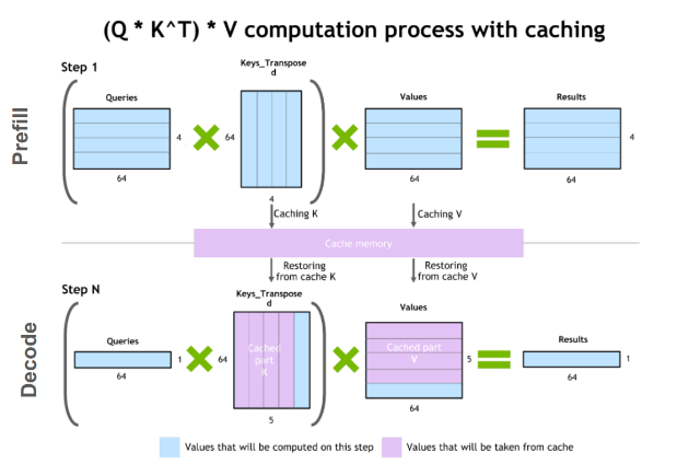
By caching, we change the computational complexity of each generation step. Instead of recomputing everything, the work at each step is dominated by attending to the growing sequence stored in the cache. This transforms the problem and is what makes generating long sequences practical.

3. The Memory Implications of the KV Cache

The "space" part of our space-time tradeoff is GPU memory, a scarce and expensive resource. The KV cache can consume a massive amount of it, sometimes even more than the model weights themselves, especially for long sequences.

Understanding how to calculate this memory usage is critical for system capacity planning. You can't schedule workloads effectively if you don't know their resource footprint.

The total memory required for the KV cache can be calculated with the following formula:

Let's break this down:

• 2: We store both a Key matrix and a Value matrix.
• num_layers: Each transformer layer has its own independent KV cache.
• batch_size: Each sequence in a batch requires its own separate cache.
• seq_len: The cache size grows linearly with the sequence length (prompt + generated tokens).
• num_kv_heads: The number of key-value heads in the attention mechanism. In standard Multi-Head Attention (MHA), this equals the number of attention heads. In optimizations like Grouped-Query Attention (GQA), this number is smaller, significantly reducing cache size.
• head_dim: The dimension of each head's key/value vector.
• bytes_per_element: The precision of the data. Typically 2 for FP16/BF16, or 1 for INT8 quantization.

The following article provides an exceptionally detailed analysis of this formula and its practical consequences.

4. Connecting to System Design

Your experience with Rudi at AWS gives you a practical understanding of resource management. The KV cache is the central resource constraint in an LLM inference scheduler.

• Capacity Planning & Admission Control: The memory calculation we just studied is the core of admission control. Before starting a new inference request, the system must check if there is enough free GPU memory to hold the model weights, existing KV caches, and the maximum potential KV cache for the new request (batch_size * max_seq_len * ...). If not, the request must be queued or rejected. This is directly analogous to the capacity allocation and QoS checks you implemented in Rudi.

• The Memory Bottleneck: As the article highlights, the generation phase of inference is often memory-bound. The speed is limited not by the GPU's computational power (FLOPs), but by its memory bandwidth—how quickly it can read the large KV cache from high-bandwidth memory (HBM) into the compute units for the attention calculation. This is why a GPU with higher memory bandwidth can sometimes outperform one with higher theoretical FLOPs for this specific workload.

• Batching Tradeoffs: To maximize GPU utilization and system throughput, we want to process requests in batches. However, since Cache Size scales linearly with batch_size, there's a direct tradeoff. A larger batch size increases throughput but consumes more memory, which in turn might force you to support a smaller maximum seq_len or require more expensive hardware. Finding the optimal batch size is a continuous balancing act.

Conclusion

In this lesson, we dissected the KV cache, the fundamental optimization that makes autoregressive generation efficient. You now understand not only its role in accelerating inference but also its profound implications for system memory and performance.

Key Takeaways:

• Role: The KV cache solves the $O(N^2)$ computational complexity of naive autoregressive generation by storing and reusing Key and Value vectors from previous tokens.
• Mechanism: It works in two phases: a higher-latency prefill for the prompt and a series of low-latency decode steps for token generation.
• Memory Impact: The cache is a major consumer of GPU memory, scaling linearly with sequence_length, batch_size, and the number of layers.
• System Bottleneck: For many common sequence lengths, LLM inference is memory-bound, limited by the bandwidth of reading the KV cache, not by raw compute power.

Next Lesson Preview

We've established that the KV cache is a per-sequence memory consumer and that batching is key to throughput. But what happens when you have a batch of requests with different sequence lengths? If you naively pad them all to the same length, you waste a tremendous amount of computation and memory.

In our next lesson, we will address this by exploring the question: Explain why batching is critical for GPU throughput and how padding impacts efficiency. We'll set the stage for advanced techniques like dynamic batching, which are crucial for building a truly efficient, high-utilization inference service.