Dynamic Batching: Balancing Latency and Throughput

Hello! Welcome to the next lesson in your preparation for the Anthropic software engineering interview.

In our last session, we established why batching is essential for LLM inference. We saw that the token-by-token decode phase is memory-bound, leaving expensive GPU compute units idle. We also identified the major flaws of naive static batching: wasted computation on padding and severe GPU underutilization due to the "straggler problem." We concluded that a dynamic, or continuous, batching approach is the only viable solution for a high-throughput system.

This lesson directly addresses the next logical step: designing such a system. We will move from the "what" to the "how," focusing on the learning outcome: Design a dynamic batching strategy that balances latency and throughput by grouping requests. Your work on the Rudi inference scheduler, particularly with priority queuing and Quality of Service (QoS), provides a strong foundation for understanding the complex trade-offs we'll discuss today.

1. The Core Idea: Iteration-Level Continuous Batching

The fundamental shift from static to continuous batching is moving from a request-level to an iteration-level scheduling mindset. Instead of waiting for an entire batch of requests to complete, the system makes scheduling decisions after every single forward pass (i.e., after each new token is generated for the active requests).

This means that at each step, the scheduler can:

• Evict requests that have just finished (by generating an <EOS> token).
• Admit new requests from the queue into the newly freed-up space.

This keeps the batch size consistently high, ensuring the GPU is always doing useful work.

Let's watch a short video that provides a clear, visual walkthrough of this dynamic process.

This simple mechanism is the heart of modern LLM serving frameworks and is the key to maximizing throughput.

2. Designing the Strategy: It's All About Tokens

How does the scheduler decide whether a new request can be added to the batch? The crucial insight is to think in terms of tokens, not requests. The primary constraints on the GPU are memory (for the KV cache) and the computational load of a forward pass. Both are functions of the number of tokens being processed.

Production systems like Hugging Face's Text Generation Inference (TGI) implement their batching logic based on token budgets. Let's explore this design.

Let's break down the core logic from that article. A dynamic batching scheduler, or router, operates on two main principles:

1. Token-Based Admission Control: A new request is admitted only if it doesn't violate the system's token capacity. The system tracks two distinct budgets:

   • MAX_BATCH_PREFILL_TOKENS (MBP): The maximum number of new tokens that can be processed in the prefill stage of a single forward pass. Prefilling is computationally intensive and creates the initial KV cache, so this limit is often determined by compute capacity and the need to keep iteration times low.
   • MAX_BATCH_TOTAL_TOKENS (MBT): The maximum number of tokens that can be held in GPU memory at once across all active requests (input tokens + generated tokens). This is primarily a memory constraint dictated by the size of the combined KV caches.

2. Stateful, Iterative Scheduling: The router's main loop continuously performs these actions:

   • Decode: Executes one decode step for the current batch of active requests.
   • Evict: Identifies and removes any requests that finished in the last step, freeing up their portion of the MAX_BATCH_TOTAL_TOKENS budget.
   • Admit & Prefill: Checks the waiting queue. It adds new requests to the batch as long as they fit within both the available MAX_BATCH_TOTAL_TOKENS and the MAX_BATCH_PREFILL_TOKENS for the current iteration. It then runs the prefill computation for these new requests.

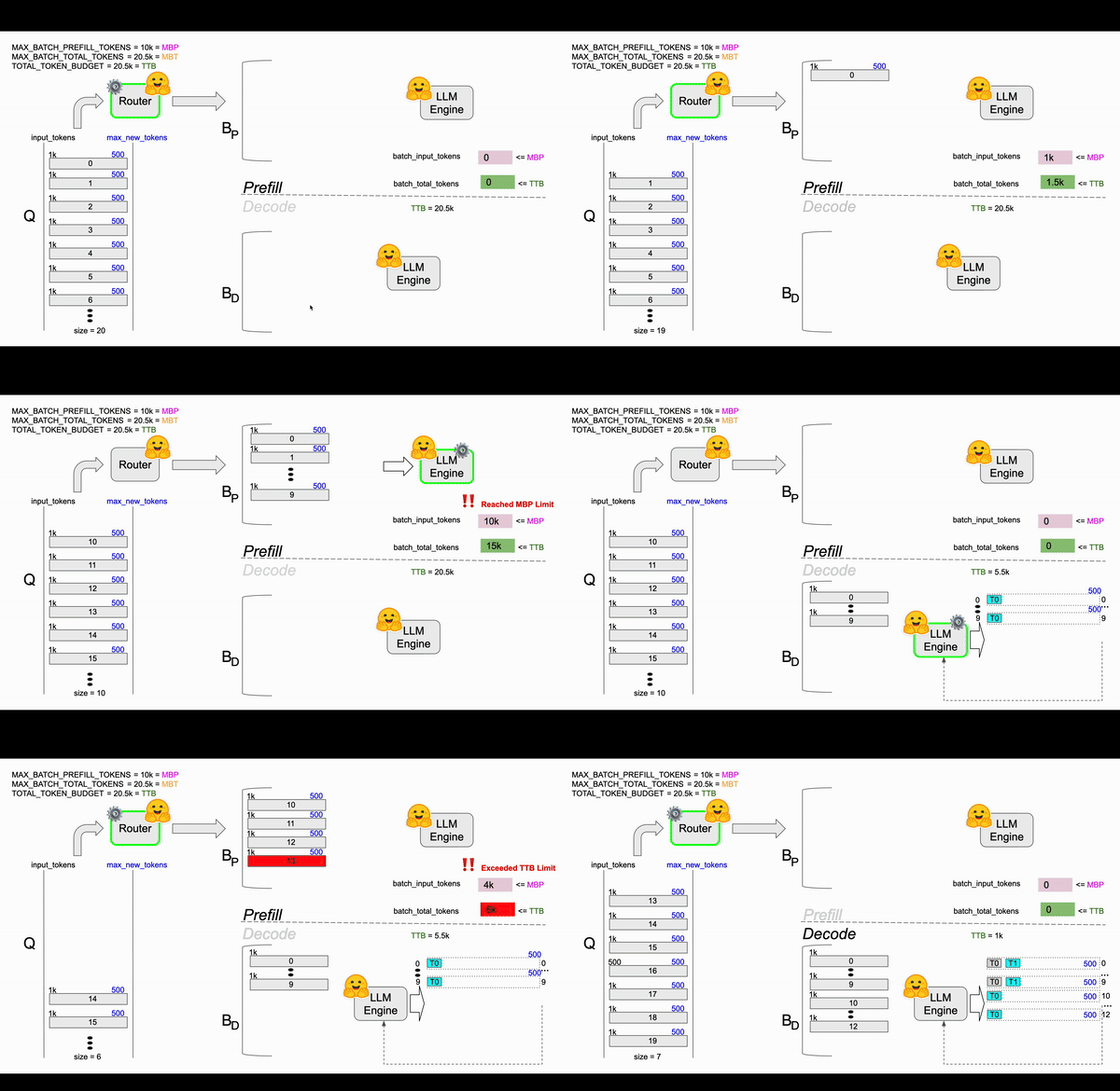
This token-budgeting approach is far more effective than simply limiting the number of requests, as it directly models the underlying hardware constraints.

3. The Central Conflict: Prefill vs. Decode Latency

The TGI design works well, but it exposes a fundamental trade-off. What happens when a new request with a very long prompt arrives?

• The prefill step for this new request will be computationally expensive and take a long time.
• If the scheduler prioritizes starting this new prefill to improve overall throughput (by getting another request active), it must pause or delay the decode steps for all other ongoing requests.

This phenomenon is called a generation stall. Users who are receiving tokens for their active requests will suddenly experience a "hiccup" or a long pause in generation. This directly impacts the time-between-tokens (TBT) latency, a critical metric for user experience.

This creates a conflict between two goals:

• High Throughput: Prefill new requests as eagerly as possible to keep the batch size high.
• Low Latency: Ensure ongoing decode steps are processed quickly and predictably.

The following graph clearly illustrates how a naive dynamic batching strategy can still fail to meet latency SLAs under increasing load due to this conflict.

4. Advanced Strategy: Chunked Prefills and Stall-Free Scheduling

How can we get the best of both worlds—high throughput and low latency? The solution lies in realizing that we don't have to prefill a long prompt all at once. This leads to the powerful technique of chunked prefills.

The core insight, as articulated in the Sarathi-Serve paper, is that "Decode batches operate in memory-bound regime leaving compute underutilized." This means a decode step doesn't use all the available GPU computation. We can use this "compute slack" to do a little bit of prefill work.

The strategy is as follows:

1. Split a large incoming prefill request into smaller, fixed-size chunks (e.g., 512 tokens each).
2. In each scheduling iteration, create a hybrid batch that contains:
   • The single decode tokens for all ongoing requests.
   • One chunk of a new prefill request.

By doing this, the scheduler ensures that every iteration has a more uniform and predictable execution time. It avoids the long stalls caused by monolithic prefills, effectively creating a "stall-free" schedule.

The following resources provide a deep dive into this advanced and highly effective strategy.

Now, for a more rigorous explanation, let's turn to the academic paper that formalized this approach.

The stall-free, chunked-prefill strategy is a sophisticated solution that directly balances latency and throughput. By ensuring that no single iteration takes an excessively long time, it maintains a low, predictable TBT for active requests while simultaneously using the GPU's spare compute cycles to make progress on admitting new requests.

Conclusion

In this lesson, we moved from the concept of dynamic batching to a concrete design. We saw that a robust strategy is token-centric and must manage the fundamental conflict between the prefill and decode phases.

Key Takeaways:

• Dynamic Batching is Token-Centric: Effective schedulers use token budgets (MAX_BATCH_PREFILL_TOKENS, MAX_BATCH_TOTAL_TOKENS) rather than request counts to manage GPU resources.
• The Core Trade-off is Prefill vs. Decode: Eagerly prefilling new requests boosts throughput but can stall ongoing decodes, spiking latency (TBT). This is the central challenge in LLM scheduling.
• Chunked Prefills are the Solution: By breaking large prefill operations into smaller chunks and creating hybrid batches (coalescing prefill chunks with decode tokens), schedulers can avoid generation stalls.
• Stall-Free Scheduling Achieves Balance: This advanced strategy yields more uniform iteration times, providing both high throughput by keeping the GPU busy and low latency by ensuring a smooth, predictable stream of tokens for users.

Next Lesson Preview

We have now designed a sophisticated strategy for scheduling requests. But this strategy—especially with its dynamic admission and eviction of requests—places immense pressure on memory management. Every request has a KV cache of a different size, and these caches are created and destroyed constantly. How do we manage this fragmented, dynamic memory landscape on the GPU without incurring huge overhead?

In our next lesson, we will tackle exactly that. We will design a memory management strategy for the KV cache to handle concurrent, variable-length requests, leading us directly to the groundbreaking PagedAttention mechanism used in systems like vLLM.