Variational Derivation of Hartree-Fock Equations

Hello! Welcome back to our module on many-body formalism.

In our last lesson, we developed the language of second quantization, which allows us to write the Hamiltonian for a system of interacting electrons in a compact and elegant way. We now have the full problem laid out:

$$\hat{H}=\sum _{\alpha ,\beta }{t}_{\alpha \beta }{c}_{\alpha }^{†}{c}_{\beta }+\frac{1}{2}\sum _{\alpha ,\beta ,\gamma ,\delta }{V}_{\alpha \beta \gamma \delta }{c}_{\alpha }^{†}{c}_{\beta }^{†}{c}_{\delta }{c}_{\gamma }$$

The challenge is that this Hamiltonian, containing the two-particle interaction term, cannot be solved exactly for any realistic system. We must resort to approximations. This lesson introduces the first, and arguably most important, of these approximations: the Hartree-Fock method.

Our goal is to derive the Hartree-Fock equations from a variational principle applied to a many-electron Hamiltonian. This will be our first application of the second quantization formalism to find an approximate ground state for an interacting system. We will see how the complex many-body problem can be reduced to a more manageable (though still challenging) set of single-particle problems.

1. The Hartree-Fock Ansatz: A Variational Approach

The core idea is to find the best possible approximation for the true many-body ground state, $|{\Psi }_0⟩$, using a simpler, more tractable trial wavefunction. The Ritz variational principle provides the criterion for "best": the trial state $|\Phi ⟩$ that minimizes the energy expectation value, $E[\Phi ]=⟨\Phi |\hat{H}|\Phi ⟩$, is the best approximation to the ground state within the class of functions from which $|\Phi ⟩$ is chosen.

What is a reasonable choice for our trial wavefunction? We need a state that is computationally simple but still respects the fundamental physics of electrons, namely the Pauli exclusion principle. The simplest such state is a single Slater determinant.

A Slater determinant describes a state where $N$ electrons occupy $N$ specific single-particle orbitals $|{\varphi }_{\lambda }⟩$ (where $\lambda =1,\dots ,N$). It is the antisymmetrized product of these orbitals:

$$|\Phi ⟩=\frac{1}{\sqrt{N!}}\det \left(\begin{array}{cccc}|{\varphi }_1{⟩}_{(1)}& |{\varphi }_2{⟩}_{(1)}& \dots & |{\varphi }_N{⟩}_{(1)}\\ |{\varphi }_1{⟩}_{(2)}& |{\varphi }_2{⟩}_{(2)}& \dots & |{\varphi }_N{⟩}_{(2)}\\ ⋮& ⋮& \ddots & ⋮\\ |{\varphi }_1{⟩}_{(N)}& |{\varphi }_2{⟩}_{(N)}& \dots & |{\varphi }_N{⟩}_{(N)}\end{array}\right)$$

In second quantization, this is written far more simply as $|\Phi ⟩=c_N^{†}{c}_{N-1}^{†}\dots c_1^{†}|0⟩$, where $c_{\lambda }^{†}$ creates an electron in the orbital $|{\varphi }_{\lambda }⟩$.

The Hartree-Fock approximation's central premise, or ansatz, is that the true ground state is well-approximated by a single Slater determinant. The "variational parameters" we will optimize are not just numbers, but the functional form of the single-particle orbitals $|{\varphi }_{\lambda }⟩$ themselves. Our goal is to find the specific set of orbitals that minimizes the total energy.

2. The Hartree-Fock Energy Functional

The first step is to calculate the expectation value of the full many-body Hamiltonian with respect to our Slater determinant trial state. This expectation value, $E[\Phi ]=⟨\Phi |\hat{H}|\Phi ⟩$, is known as the Hartree-Fock energy functional.

The following reading walks through this calculation in detail. It starts from the first-quantized Hamiltonian and a Slater determinant, and carefully evaluates the expectation values of the one-body (kinetic + external potential) and two-body (Coulomb interaction) terms.

The calculation yields the celebrated Hartree-Fock energy functional:

$$E_{HF}[\{{\varphi }_{\lambda }\}]=\sum _{\lambda =1}^N{I}_{\lambda }+\frac{1}{2}\sum _{\lambda ,\mu =1}^N(J_{\lambda \mu }-K_{\lambda \mu })$$

Let's break down these terms:

• $I_{\lambda }=⟨{\varphi }_{\lambda }|{\hat{h}}_1|{\varphi }_{\lambda }⟩$: The one-electron energy, consisting of the kinetic energy and the potential energy from the ionic lattice for an electron in orbital ${\varphi }_{\lambda }$.
• $J_{\lambda \mu }=⟨{\varphi }_{\lambda }{\varphi }_{\mu }|\frac{e^2}{4\pi {ϵ}_0|\mathbf{r}-{\mathbf{r}}^{\prime }|}|{\varphi }_{\lambda }{\varphi }_{\mu }⟩$: The direct integral. This term represents the classical electrostatic repulsion energy between the charge cloud $|{\varphi }_{\lambda }(\mathbf{r}){|}^2$ and the charge cloud $|{\varphi }_{\mu }({\mathbf{r}}^{\prime }){|}^2$.
• $K_{\lambda \mu }=⟨{\varphi }_{\lambda }{\varphi }_{\mu }|\frac{e^2}{4\pi {ϵ}_0|\mathbf{r}-{\mathbf{r}}^{\prime }|}|{\varphi }_{\mu }{\varphi }_{\lambda }⟩$: The exchange integral. This term has no classical analogue. It arises purely from the antisymmetry of the fermionic wavefunction. Notice the swapped orbitals in the ket. The exchange term is non-zero only for electrons with the same spin ($K_{\lambda \mu }\propto {\delta }_{{\sigma }_{\lambda },{\sigma }_{\mu }}$). Since $K_{\lambda \mu }>0$, it lowers the energy. This "exchange interaction" favors aligning spins to minimize Coulomb repulsion, as the Pauli principle keeps same-spin electrons spatially separated. This is the origin of Hund's first rule in atoms.

3. Deriving the Hartree-Fock Equations

Now that we have the energy functional, we must find the orbitals $\{{\varphi }_{\lambda }\}$ that minimize it. We can't just take the derivative, because the orbitals must remain orthonormal ($⟨{\varphi }_{\lambda }|{\varphi }_{\mu }⟩={\delta }_{\lambda \mu }$). This is a constrained optimization problem, which we solve using the method of Lagrange multipliers.

We seek to make the following functional stationary with respect to variations in the orbitals:

$$\mathcal{L}[\{{\varphi }_{\lambda }\}]=E_{HF}[\{{\varphi }_{\lambda }\}]-\sum _{\lambda ,\mu =1}^N{ϵ}_{\lambda \mu }(⟨{\varphi }_{\lambda }|{\varphi }_{\mu }⟩-{\delta }_{\lambda \mu })$$

Here, ${ϵ}_{\lambda \mu }$ are the Lagrange multipliers. Setting the functional derivative $\frac{\delta \mathcal{L}}{\delta {\varphi }_{\lambda }^{\ast }(\mathbf{r})}=0$ leads to the Hartree-Fock equations.

The following reading provides the final steps of the derivation.

After some algebra, we arrive at the canonical Hartree-Fock equations:

$$\left(-\frac{{\hslash }^2}{2m}{\nabla }^2+V_{ext}(\mathbf{r})\right){\varphi }_{\lambda }(\mathbf{r})+\left(\sum _{\mu =1}^N\int d{\mathbf{r}}^{\prime }\frac{e^2|{\varphi }_{\mu }({\mathbf{r}}^{\prime }){|}^2}{4\pi {ϵ}_0|\mathbf{r}-{\mathbf{r}}^{\prime }|}\right){\varphi }_{\lambda }(\mathbf{r})-\sum _{\mu =1}^N\left(\int d{\mathbf{r}}^{\prime }\frac{e^2{\varphi }_{\mu }^{\ast }({\mathbf{r}}^{\prime }){\varphi }_{\lambda }({\mathbf{r}}^{\prime })}{4\pi {ϵ}_0|\mathbf{r}-{\mathbf{r}}^{\prime }|}\right){\varphi }_{\mu }(\mathbf{r}){\delta }_{{\sigma }_{\lambda },{\sigma }_{\mu }}={ϵ}_{\lambda }{\varphi }_{\lambda }(\mathbf{r})$$

(It can be shown that the matrix of Lagrange multipliers ${ϵ}_{\lambda \mu }$ can be diagonalized, giving the eigenvalues ${ϵ}_{\lambda }$).

This equation looks formidable, but it has a clear structure. It's a single-particle Schrödinger-like equation for each orbital ${\varphi }_{\lambda }$. Let's define the Fock operator $\hat{F}$ such that $\hat{F}{\varphi }_{\lambda }={ϵ}_{\lambda }{\varphi }_{\lambda }$. It contains:

1. Kinetic energy and external potential: $-\frac{{\hslash }^2}{2m}{\nabla }^2+V_{ext}(\mathbf{r})$.
2. The Hartree Potential (Direct Term): $V_H(\mathbf{r})={\sum }_{\mu }\int d{\mathbf{r}}^{\prime }\frac{e^2|{\varphi }_{\mu }({\mathbf{r}}^{\prime }){|}^2}{4\pi {ϵ}_0|\mathbf{r}-{\mathbf{r}}^{\prime }|}$. This is a local potential energy term. It represents the average electrostatic potential at point $\mathbf{r}$ created by the charge distribution of all electrons in the system.
3. The Fock Potential (Exchange Term): This is the last term on the left. Unlike the Hartree term, it's a non-local integral operator. It doesn't multiply ${\varphi }_{\lambda }(\mathbf{r})$ by a function; it swaps ${\varphi }_{\lambda }$ with ${\varphi }_{\mu }$ inside the integral. This exchange term acts as an effective attractive potential between electrons of the same spin.

The video below gives an excellent and concise summary of the entire approximation and the resulting equations.

4. Solving the Equations: The Self-Consistent Field (SCF) Method

A critical feature of the Hartree-Fock equations is their non-linearity. The Fock operator $\hat{F}$, which determines the orbitals ${\varphi }_{\lambda }$, itself depends on those very same orbitals through the Hartree and Fock potentials.

This "chicken-and-egg" problem means we cannot solve the equations directly. Instead, we must use an iterative approach called the Self-Consistent Field (SCF) method.

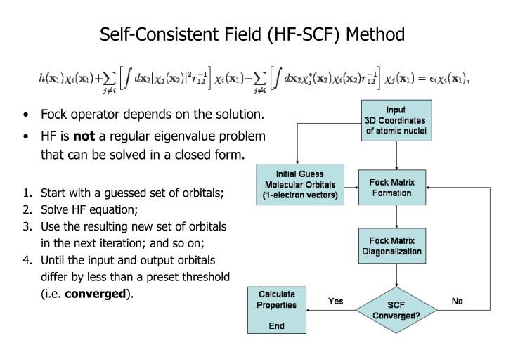
The SCF procedure works as follows:

1. Initial Guess: Make an initial guess for the set of orbitals $\{{\varphi }_{\lambda }^{(0)}\}$.
2. Build Fock Operator: Use the current set of orbitals $\{{\varphi }_{\lambda }^{(i)}\}$ to construct the Hartree and Fock potentials, and thus the Fock operator ${\hat{F}}^{(i)}$.
3. Solve Eigenvalue Problem: Solve the eigenvalue equation ${\hat{F}}^{(i)}{\varphi }_{\lambda }^{(i+1)}={ϵ}_{\lambda }^{(i+1)}{\varphi }_{\lambda }^{(i+1)}$ to obtain a new, improved set of orbitals $\{{\varphi }_{\lambda }^{(i+1)}\}$.
4. Check for Convergence: Compare the new orbitals/energies with the previous ones. If they are the same within a certain tolerance, self-consistency is reached, and the process stops.
5. Iterate: If not converged, mix the old and new orbitals to create the input for the next iteration ($\{{\varphi }_{\lambda }^{(i+1)}\}$ becomes the new $\{{\varphi }_{\lambda }^{(i)}\}$) and go back to step 2.

This iterative process finds a set of orbitals that are eigenfunctions of the very potential they themselves generate—a self-consistent field.

Test your understanding!

The exchange term $K_{\lambda\mu}$ lowers the total energy $E_{HF}$. Why does this term lead to Hund's first rule, which states that for a given electron configuration, the term with maximum spin multiplicity has the lowest energy?

Show answer

The exchange integral $K_{\lambda\mu}$ is non-zero only if the orbitals $\phi_\lambda$ and $\phi_\mu$ have the same spin. The total energy is lowered by a sum over all pairs $(\lambda, \mu)$ of $-K_{\lambda\mu}$. To make the energy as low as possible, we want to maximize the number of pairs with the same spin, as each such pair contributes a negative energy term. This is achieved by aligning as many electron spins as possible (maximizing spin multiplicity), up to the limit imposed by the Pauli principle for a given shell.

Conclusion

In this lesson, we have performed the foundational derivation of many-body theory. By applying the variational principle to a single Slater determinant, we reduced the intractable full Hamiltonian to a set of coupled, single-particle, non-linear equations—the Hartree-Fock equations.

Key Takeaways:

• The Hartree-Fock method approximates the many-body ground state with a single Slater determinant, the simplest wavefunction that respects Fermi statistics.
• The optimal orbitals are found by minimizing the expectation value of the energy using the variational principle.
• The resulting Hartree-Fock equations describe single electrons moving in an effective potential created by the other electrons. This potential has two parts:
  • A local Hartree term: classical Coulomb repulsion from the average electron density.
  • A non-local exchange term: a purely quantum mechanical effect due to the Pauli principle, which lowers the energy for electrons with parallel spins.
• The non-linear nature of the equations requires an iterative Self-Consistent Field (SCF) procedure for their solution.

The Hartree-Fock state provides a powerful "zeroth-order" picture of the electronic ground state. The orbital energies ${ϵ}_{\lambda }$ can be related (via Koopmans' theorem) to the energies needed to add or remove an electron, which are quantities measured in photoemission and inverse photoemission spectroscopy, experiments with which you have some familiarity. However, it is still an approximation that neglects electron correlation.

Preview of the Next Lesson

The Hartree-Fock method gives us an approximate ground state and a set of single-particle orbitals. What about the excitations of the system? How do we describe the behavior of an added electron or a "hole" left behind? The next lesson will introduce the central mathematical tool for this: the single-particle Green's function. We will define this function and see how its properties, particularly its poles in the complex frequency plane, relate to the quasiparticle excitations of the interacting system.