Checking Binomial Model Assumptions in Repeated Trials

Hello! In the previous lesson, you used the complement rule to find the chance of at least one success. You also saw that multiplying failure probabilities required an assumption about how the attempts relate to one another. This module takes the next step: instead of asking only whether any success occurs, we will study the number of successes in a set of attempts.

Before calculating binomial probabilities, you need to know when a binomial model is appropriate. Today you will check four assumptions against the way observations were actually generated. That model check will matter later when you assess whether an observed group rate is surprising or could plausibly arise by chance.

Define the trial before checking the model

Suppose you observe a fixed set of attempts and classify each one as a success or a failure. Write $Y_i=1$ if attempt $i$ succeeds and $Y_i=0$ otherwise. The total number of successes is

A binomial model describes this count, $X$, when the attempts meet four conditions. The mnemonic BINS keeps them together:

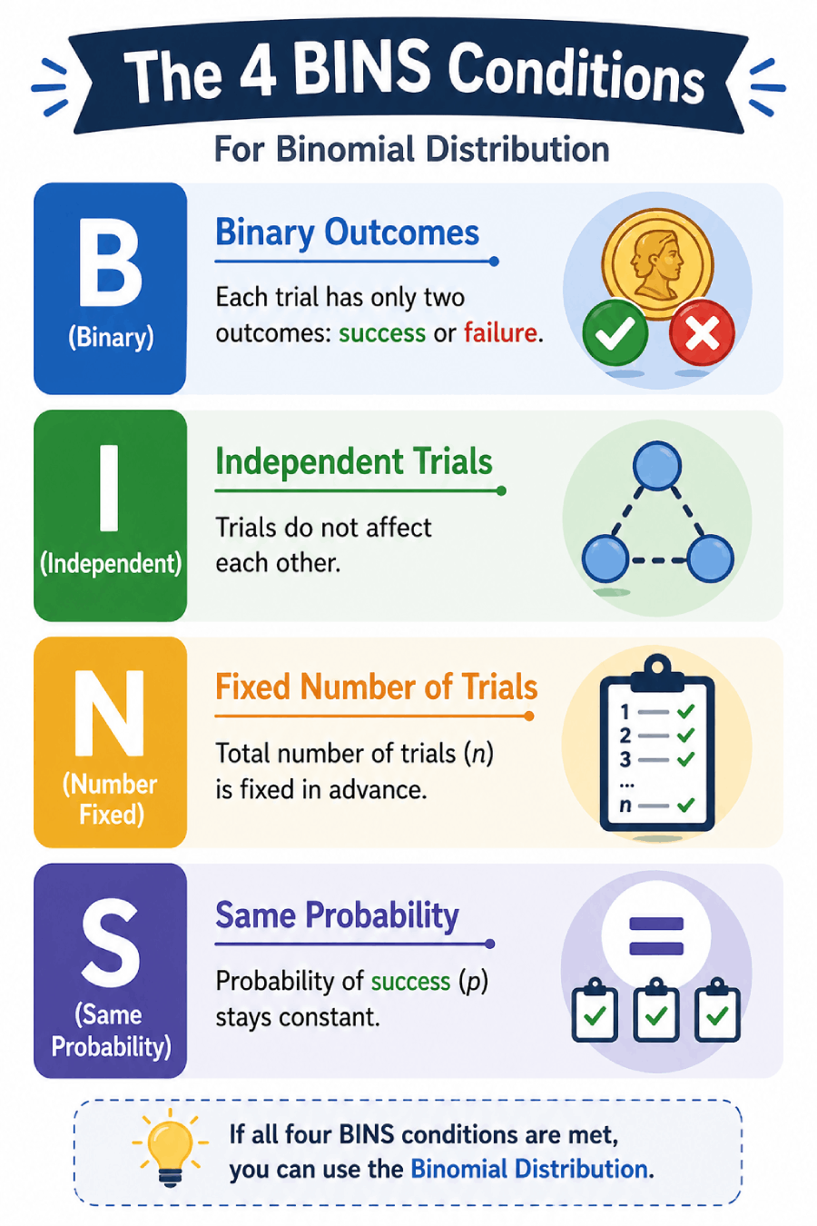
“Binary” refers to the classification you count, not necessarily to everything that can happen during a trial. A die has six possible faces, but “rolled a three or four” versus “did not” is a valid yes/no classification. If you roll it a predetermined 16 times, with rolls that do not influence one another and the same chance of a three or four each time, the count of successes fits a binomial model.

The fixed-number condition concerns the number of attempts, not the number of successes. “Roll 16 times and count the sixes” has a fixed number of trials. “Roll until the third six appears” does not: you know the final success count, but the number of rolls is unknown in advance.

Watch how these distinctions are made in the following examples.

A fixed duration is not automatically a fixed number of trials. Counting events that occur during five minutes, for example, does not specify five or any other predetermined number of yes/no attempts. By contrast, observing exactly 50 arrivals and asking whether each meets a criterion gives 50 trials, even if the time needed to observe them varies.

Independence and constant probability are separate checks

For independence, learning one trial’s result must not change the probability assigned to another trial’s result. In the notation from the earlier conditional-probability lesson, independent trials satisfy, for example,

For constant probability, there must be one value $p$ such that each trial has success probability $p$. Neither condition guarantees the other.

Imagine two independent attempts, one with success probability $0.2$ and the other with success probability $0.8$. The first result tells you nothing about the second, so independence holds. But there is no single success probability $p$ shared by both attempts. Substituting their average, $0.5$, into a binomial model would not repair that: the actual chance that both succeed is $0.2(0.8)=0.16$, whereas two independent trials each with probability $0.5$ would give $0.25$.

Conversely, suppose two recorded attempts always copy the same underlying yes/no outcome, which has a $0.3$ chance of success. Each recorded attempt has the same marginal success probability, $0.3$. Yet after the first succeeds, the second succeeds with probability $1$, not $0.3$. The probabilities match across attempts, but the attempts are dependent.

These are practical modeling questions, not properties you can establish just by seeing a Boolean column. Conditions might change over time, producing different success probabilities. Observations from the same batch might share an influence, producing dependence. The fact that you can calculate a rate from the data does not, by itself, establish either assumption.

The video gives further contrasts, including attempts with changing difficulty and a count collected over a fixed time.

Sampling without replacement: an instructive failure

Consider a collection of 30 items, six of which have a specified tag. You randomly draw two items without replacement and count how many are tagged. The outcome is binary for each draw, and the number of draws is fixed. But the first result changes what remains for the second:

The first-draw probability is $6/30$. Interestingly, the unconditional probability that the second draw is tagged is also $6/30$, by symmetry. Equal unconditional probabilities for the two draw positions do not make the draws independent: their conditional probabilities reveal the dependence. This is why it helps to check independence separately from a shared marginal rate.

The following reading formalizes the model and discusses both this kind of small collection and the approximation often used for a much larger population.

Sampling without replacement from a small collection is not exactly binomial. When the number drawn is small relative to a very large population, removing one item changes the composition only slightly, and a binomial model can be a useful approximation. “Approximately binomial” is a modeling judgment, not a claim that the draws have become exactly independent. A small sampling fraction also does not resolve other possible sources of dependence, such as items arriving in related batches.

You can see the conditional probabilities directly in a short simulation. Here item IDs 0 through 5 are tagged, and each simulated pair is drawn without replacement:

import numpy as np

rng = np.random.default_rng(42)
draws = np.array([
    rng.choice(30, size=2, replace=False)
    for _ in range(50_000)
])

tagged = draws < 6

print("Second tagged, overall:", tagged[:, 1].mean())
print("Second tagged | first tagged:",
      tagged[tagged[:, 0], 1].mean())
print("Second tagged | first untagged:",
      tagged[~tagged[:, 0], 1].mean())

The first output should be near $6/30=0.2$; the next two should be near $5/29$ and $6/29$, respectively. Simulation makes the consequence of the specified drawing procedure visible. It cannot establish that a real dataset was collected by that procedure; that requires knowledge of how the observations were sampled.

Make the model check explicit

Before treating a count as binomial, state what one trial is, what qualifies as success, and what $X$ counts. Then ask whether:

1. every trial can be classified as success or failure;
2. the number $n$ of trials was set in advance;
3. trial outcomes are reasonably independent; and
4. the success probability can reasonably be treated as the same $p$ on every trial.

A count of successes in a predetermined set of independent, identically conducted attempts meets the checks. A count accumulated until a target number of successes does not meet the fixed-$n$ check. A sample drawn without replacement from a small collection fails exact independence; a sample drawn from a much larger population may justify an approximation. Independent attempts conducted under substantially different conditions can fail the common-$p$ check.

The aim is not to reject every useful model because reality is imperfect. It is to distinguish which assumptions are exact by design, which are defensible approximations, and which are unsupported. That distinction becomes especially important when a numerical probability will later be interpreted as evidence that a group’s observed rate is unusual.

Key takeaways

A binomial model applies to a count of successes across a fixed number of binary-classified trials that are independent and share one success probability. Independence and equal probability are distinct requirements; checking only the observed rate does not establish either one. Sampling without replacement illustrates the difference between an exact binomial model and a potentially useful approximation.

In the next lesson, you will use these conditions to derive the binomial probability formula: the multiplication rule gives the probability of one particular success pattern, and combinations count how many patterns yield the same total.