Shor's Algorithm vs. General Number Field Sieve: Complexity and Speedup

Recommended resources

The freely available resources this lesson will direct you to.

Hello! Welcome to the final lesson in our module on foundational quantum algorithms.

In our previous lesson, we successfully constructed the complete quantum circuit for the period-finding subroutine. We saw how to integrate the modular exponentiation oracle, which we had built earlier, into the Quantum Phase Estimation (QPE) framework to extract the period $r$ of a function $f (x) = a^{x} (mod N)$ .

Today, we will take a step back and analyze the "so what?" of this achievement. We will assess the computational resources required by this quantum procedure and compare them against the most powerful classical methods. This will allow us to precisely quantify the quantum advantage of Shor's algorithm.

Our learning outcome is to compare the computational complexity of the quantum period-finding subroutine in Shor's algorithm with that of the General Number Field Sieve, identifying the source of the exponential speedup.

This lesson will bridge the gap between quantum circuit design and computational complexity theory, providing the capstone for our study of Shor's algorithm.

1. Complexity Analysis of Shor's Algorithm

To analyze the efficiency of an algorithm, we study how the number of elementary operations scales with the size of the input. For factoring an integer $N$ , the input size is the number of bits required to represent $N$ , which is $n = ⌈ lo g_{2} N ⌉$ . An "efficient" algorithm is one whose runtime is a polynomial function of $n$ .

Shor's algorithm is a hybrid quantum-classical algorithm. Let's break it down and analyze the complexity of each stage.

Shor's Algorithm and the Quantum Fourier Transform

This document provides a concise overview of the complexity of Shor's algorithm and introduces the relevant complexity classes. It will help ground our analysis.

Please read the 'Introduction' (first page) and the 'Conclusion' (Section 7). The introduction defines key complexity classes like BQP (Bounded-error Quantum Polynomial time), which is where Shor's algorithm lives. The conclusion explicitly states the overall complexity of the algorithm. We will derive this result step-by-step.

As you've just read, Shor's algorithm runs in polynomial time, placing the factoring problem in the complexity class BQP. Let's see where that result comes from.

Algorithm Breakdown:

Classical Pre-processing:
- Check if $N$ is even, prime, or a prime power. These checks can be performed efficiently on a classical computer in polynomial time, specifically $O (n^{3})$ or better.
- Choose a random $a < N$ and compute $gcd (a, N)$ . The Euclidean algorithm is very efficient, running in $O (n^{2})$ time.
Quantum Period-Finding Subroutine: This is the core of the algorithm, which we built in the last lesson. It uses a counting register of $t$ qubits and a state register of $n$ qubits. We typically choose $t \approx 2 n$ .
- State Preparation: Applying Hadamard gates to the $t$ qubits in the counting register takes $O (t) = O (n)$ gates.
- Modular Exponentiation: This is the most computationally intensive part of the quantum circuit. It implements the mapping $∣ x ⟩ ∣ y ⟩ \mapsto ∣ x ⟩ ∣ y \cdot a^{x} (mod N)⟩$ . Using the method of repeated squaring, this requires $O (n)$ sequential modular multiplications. Each modular multiplication of $n$ -bit numbers can be implemented with a circuit of size $O (n^{2})$ . Thus, the total complexity of this step is $O (n^{3})$ .
- Inverse Quantum Fourier Transform (QFT⁻¹): The QFT circuit on $t$ qubits consists of $t$ Hadamard gates and $t (t - 1) /2$ controlled-rotation gates. Its complexity is $O (t^{2}) = O (n^{2})$ .
Classical Post-processing:
- Measurement: Reading out the $t$ qubits takes $O (t) = O (n)$ time.
- Continued Fractions Algorithm: This classical algorithm takes the measurement outcome $m$ and finds the best rational approximation to $m / 2^{t}$ . Its complexity is $O (n^{3})$ .

Summing these up, the overall complexity of a single run of Shor's algorithm is dominated by the modular exponentiation and continued fractions steps, yielding a total complexity of $O (n^{3})$ . This is a polynomial-time algorithm.

2. The Classical Competitor: General Number Field Sieve (GNFS)

To appreciate the power of Shor's algorithm, we must compare it to the best-known classical factoring algorithm. For numbers larger than about 100 digits, this is the General Number Field Sieve (GNFS).

A Beginner's Guide To The General Number Field Sieve

Let's briefly introduce the classical champion. This paper provides a high-level overview of the GNFS.

Please read the 'Introduction' (Section I) and the 'Conclusion' (Section IV). You don't need to dive into the mechanics of the algorithm itself. The key is to understand its status as the best classical method and to note the description of its performance.

The GNFS, like many factoring algorithms, is based on finding a non-trivial congruence of squares, $x^{2} \equiv y^{2} (mod N)$ . Its innovation lies in using sophisticated algebraic number theory to find such a congruence much faster than previous methods.

The crucial point for our comparison is its computational complexity. The runtime of GNFS is given by a formula of the form:
$L_{N} [α, c] = exp (c (lo g N)^{α} (lo g lo g N)^{1 - α})$
For GNFS, $α = 1/3$ and $c \approx 1.923$ . Substituting $n = lo g N$ , the complexity is:
$O (exp (c \cdot n^{1/3} (lo g n)^{2/3}))$
This is classified as sub-exponential, but it is crucially super-polynomial. It grows faster than any polynomial in $n$ , but slower than a pure exponential like $e^{n}$ . This is why factoring is considered "hard" for classical computers.

3. The Quantum Advantage: A Tale of Two Complexities

Now we can directly compare the scaling of the two algorithms:

Shor's Algorithm: $O (n^{3})$ — Polynomial
GNFS: $O (exp (c \cdot n^{1/3} (lo g n)^{2/3}))$ — Sub-exponential

The difference is dramatic. For a polynomial algorithm, doubling the input size increases the runtime by a constant factor (e.g., $2^{3} = 8$ ). For a sub-exponential algorithm, the runtime increases much more severely.

The following graphs visualize this difference starkly.

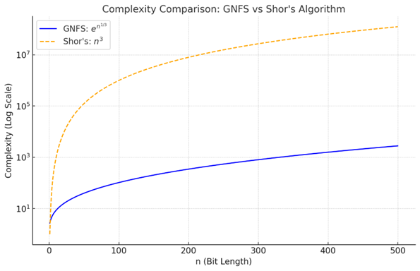
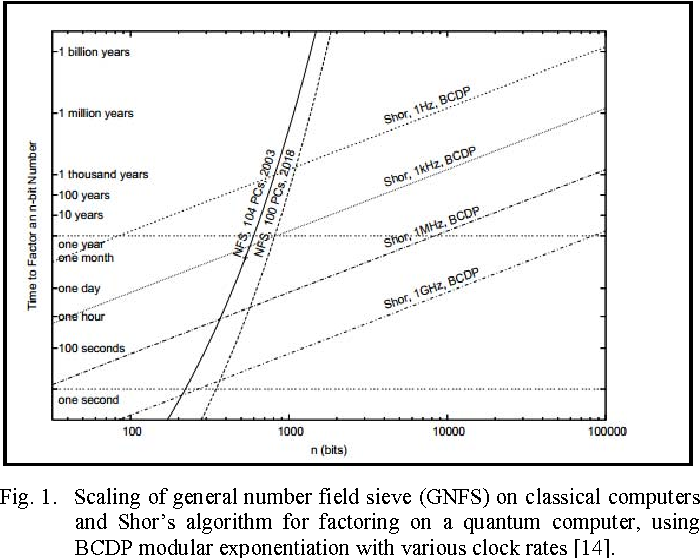
Caption: A log-scale plot comparing the asymptotic complexity of Shor's algorithm (polynomial, $n^3$) and a simplified representation of the General Number Field Sieve (sub-exponential, $\exp(n^{1/3})$). As the number of bits $n$ increases, the resources required by GNFS grow far more rapidly than for Shor's algorithm.

Caption: A log-log plot showing projected time to factor an $n$-bit number. The line for GNFS (classical) shows a steep increase, while the lines for Shor's algorithm (quantum) are much flatter, illustrating the practical impact of the polynomial vs. sub-exponential scaling. The different lines for Shor's correspond to hypothetical quantum computer clock speeds.

This vast difference in scaling is what we mean by an exponential speedup.

Identifying the Source of the Speedup

Where does this incredible advantage come from? It's a combination of two uniquely quantum features: superposition and interference.

Quantum Algorithms - Ronald de Wolf

To understand the source of the speedup, it's helpful to revisit the high-level concepts of quantum parallelism and interference. This lecture by Ronald de Wolf provides a clear, conceptual explanation.

Please watch these two short segments: 'Quantum Parallelism and Interference' (13:35 - 16:45): This explains why superposition alone ('quantum parallelism') is not enough. 'Sketch of Shor's Algorithm: Quantum Period-Finding using QFT' (22:37 - 25:21): This shows how the QFT uses interference to extract the period, which is the crucial second step. Focus on the distinction between creating the superposition of all function values and the act of extracting the global property (the period) from that superposition.

As the video explains, the speedup is not simply from "trying all answers at once."

Quantum Parallelism: The modular exponentiation step creates the state:
$\frac{1}{2 ^{t}} x = 0 \sum 2^{t} - 1 ∣ x ⟩ ∣ a^{x} (mod N)⟩$
In a sense, we have computed all $2^{t}$ values of the function $f (x) = a^{x} (mod N)$ in a single operation. This is the power of superposition. However, if we were to measure this state, we would get just one random pair $∣ x, a^{x} (mod N)⟩$ , which is useless. This is no better than classical computation.
Quantum Fourier Transform and Interference: The magic happens when we apply the QFT⁻¹ to the first register. The state we created is periodic with period $r$ . The QFT is a quantum analogue of the classical Fourier transform, which is exceptionally good at finding periodicities (frequencies) in signals. The QFT causes all the different computational paths in the superposition to interfere. This interference is constructive for states that are related to the period $r$ and destructive for all other states.

When we measure the first register after the QFT, the probability distribution is sharply peaked at values $m$ such that $m / 2^{t} \approx s / r$ for some integer $s$ . The QFT has efficiently extracted the global property (the period) of the function from the superposition, a task that is classically intractable because it would require evaluating the function at many points to detect the pattern.

In short:

Source of Speedup = Quantum Parallelism + Efficient Period Extraction via QFT.
The QFT provides an efficient way ( $O (n^{2})$ gates) to perform a Fourier transform on an exponentially large ( $2^{n}$ -dimensional) state vector, a feat with no known efficient classical equivalent.

Conclusion

This lesson marks the culmination of our study of Shor's algorithm, the crown jewel of the early era of quantum algorithms.

Key Takeaways:

Shor's algorithm for factoring an $n$ -bit integer has a computational complexity of $O (n^{3})$ , making it a polynomial-time algorithm that belongs to the class BQP.
The best-known classical algorithm, the General Number Field Sieve (GNFS), has a sub-exponential complexity of $O (exp (c \cdot n^{1/3} (lo g n)^{2/3}))$ .
The difference between polynomial and sub-exponential scaling gives Shor's algorithm an exponential speedup over classical methods for large $n$ .
The source of this speedup is twofold: quantum parallelism allows for the creation of a state encoding the function $a^{x} (mod N)$ over all $x$ , and the Quantum Fourier Transform efficiently extracts the function's period through massive constructive and destructive interference.

You have now analyzed one of the most profound results in quantum computation, from the underlying number theory to the circuit implementation and its complexity-theoretic implications.

Preview of the Next Module:

Shor's algorithm and the others we've studied (Deutsch-Jozsa, Grover's) are designed for idealized, error-free quantum computers. In the next module, "Variational Algorithms and Hamiltonian Simulation," we will shift our focus to algorithms designed for the noisy, intermediate-scale quantum (NISQ) devices that exist today. We will explore heuristic approaches like the Variational Quantum Eigensolver (VQE) and the Quantum Approximate Optimization Algorithm (QAOA), which represent a different paradigm of quantum algorithm design.