Sharpe Ratio: Measuring Risk-Adjusted Returns

Hello! Welcome to the next lesson in our module on advanced performance and risk-adjusted returns.

In the previous lesson, we established how to quantify risk using standard deviation to measure the volatility of projected returns. Knowing an investment's potential return is one half of the equation; understanding its risk is the other. Now, it's time to put them together.

Today's learning outcome is to calculate the Sharpe ratio to assess risk-adjusted returns. This metric, developed by Nobel laureate William F. Sharpe, is a cornerstone of modern finance. It provides a single, powerful number to answer the question: "Am I being adequately compensated for the risk I'm taking?" For you, mastering the Sharpe ratio is a key step toward comparing diverse investment opportunities, like a stable rental in one city versus a more speculative one in another, on an apples-to-apples basis.

1. Beyond Returns: The Need for a Risk-Adjusted Metric

As we've discussed, relying solely on returns can be misleading. An investment that returns 10% with wild swings is not necessarily better than one that returns 8% with steady, predictable gains. The Sharpe ratio was designed to capture this exact intuition.

To see why this is so important, let's watch a short video that brilliantly illustrates the concept.

As the video explains, the investment with higher volatility is more painful to hold, gives you less confidence in its future performance, and exposes you to liquidity risk—the danger of needing to sell at a loss. This is why we need a metric that rewards returns but penalizes risk.

2. Deconstructing the Sharpe Ratio

The Sharpe ratio elegantly combines return and risk into one formula.

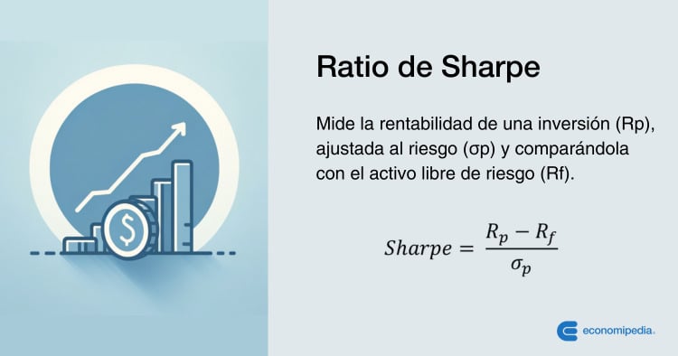
The formula is:
$\text{Sharpe Ratio}=\frac{R_p-R_f}{{\sigma }_p}$
Let's break down its components, which should look familiar:

• $R_p$ (Return of Portfolio): This is the average expected return of your investment. In our case, this would be the average projected annual return from our real estate model.
• $R_f$ (Risk-Free Rate): This is the return you could theoretically get on an investment with zero risk. For our purposes, we'll use the yield on a Spanish 10-year government bond (Bono del Estado a 10 años). This is a standard benchmark for risk-free returns in Spain. A rational investor would only take on risk if they expect to earn more than this rate.
• $R_p-R_f$ (Excess Return): This is the numerator of the formula and represents your risk premium—the extra return you get as a reward for taking on risk instead of just buying a safe government bond.
• ${\sigma }_p$ (Standard Deviation of Portfolio's Return): This is the denominator. It's the investment's volatility, which we learned to calculate in the last lesson. It represents the "cost" of your excess return in terms of risk.

In essence, the Sharpe ratio tells you how much excess return you are getting for each unit of risk you take.

For a more detailed breakdown of these components, the following reading is highly recommended.

3. Calculating the Sharpe Ratio for a Real Estate Investment

Let's apply this to the two hypothetical properties from our last lesson. Assume the current risk-free rate (Spanish 10-year bond yield) is 3.0%.

Property A (Stable)

• Average Projected Return ($R_p$): 6.9%
• Volatility (${\sigma }_p$): 0.96%
• Risk-Free Rate ($R_f$): 3.0%

${\text{Sharpe Ratio}}_A=\frac{0.069-0.030}{0.0096}=\frac{0.039}{0.0096}\approx 4.06$

Property B (Volatile)

• Average Projected Return ($R_p$): 5.8% (let's use the actual mean from the previous lesson's code)
• Volatility (${\sigma }_p$): 5.50%
• Risk-Free Rate ($R_f$): 3.0%

${\text{Sharpe Ratio}}_B=\frac{0.058-0.030}{0.0550}=\frac{0.028}{0.0550}\approx 0.51$

The results are stark. Property A has a Sharpe ratio of 4.06, while Property B's is only 0.51. This tells us that Property A provides a much higher return for the level of risk involved. Even if Property B had a slightly higher average return, its massive volatility would still result in a much lower Sharpe ratio, making it the inferior choice from a risk-adjusted perspective.

4. Interpretation and Context

A Sharpe ratio is most useful for comparison, but some general benchmarks can provide context:

• < 1.0: Considered suboptimal. The returns don't adequately compensate for the risk.
• 1.0 – 1.99: Considered good.
• 2.0 – 2.99: Considered very good.
• > 3.0: Considered excellent.

A negative Sharpe ratio indicates that the investment's return is less than the risk-free rate. You'd be taking on risk to get a worse return than a government bond—a clear signal to avoid the investment.

The following resource provides an example of this exact situation in the Spanish real estate context.

Annualization

When dealing with stock market data, which is often daily or monthly, the Sharpe ratio is typically annualized to allow for fair comparisons. This is done by multiplying the calculated ratio by the square root of the number of periods in a year (e.g., $\sqrt{252}$ for daily data, $\sqrt{12}$ for monthly).

For our real estate projections, since we are using annual projected returns, the resulting Sharpe ratio is already annualized. No further conversion is necessary.

5. Python Implementation

Let's write a Python function to automate this calculation. It will build upon the code from our previous lesson.

import numpy as np

def calculate_sharpe_ratio(projected_returns, risk_free_rate):
    """
    Calculates the Sharpe Ratio for a series of projected annual returns.
    
    Args:
        projected_returns (list or np.array): A list of projected annual returns.
        risk_free_rate (float): The annual risk-free rate.
        
    Returns:
        float: The annualized Sharpe Ratio.
    """
    
    # Calculate the mean of the projected returns
    mean_return = np.mean(projected_returns)
    
    # Calculate the sample standard deviation (volatility)
    # ddof=1 is used for sample standard deviation
    std_dev = np.std(projected_returns, ddof=1)
    
    # Avoid division by zero if there is no volatility
    if std_dev == 0:
        # If returns are constant, Sharpe is infinite if mean > risk_free_rate,
        # otherwise it's arguably 0 or undefined. We'll return 0.
        return 0.0 if mean_return <= risk_free_rate else np.inf

    # Calculate the excess return
    excess_return = mean_return - risk_free_rate
    
    # Calculate the Sharpe Ratio
    sharpe_ratio = excess_return / std_dev
    
    return sharpe_ratio

# --- Example Usage ---

# Data from previous lesson
property_A_returns = [0.065, 0.070, 0.055, 0.080, 0.075] 
property_B_returns = [0.02, 0.12, 0.05, 0.11, -0.01]

# Set the risk-free rate (e.g., Spanish 10-year bond yield)
spanish_rf_rate = 0.03

# Calculate Sharpe Ratios
sharpe_A = calculate_sharpe_ratio(property_A_returns, spanish_rf_rate)
sharpe_B = calculate_sharpe_ratio(property_B_returns, spanish_rf_rate)

print("--- Risk-Adjusted Return Analysis ---")
print(f"Property A Sharpe Ratio: {sharpe_A:.2f}")
print(f"Property B Sharpe Ratio: {sharpe_B:.2f}")

This code confirms our manual calculations and demonstrates how easily you can compare the risk-adjusted performance of different investment opportunities.

6. Advanced Implications: Leverage and Diversification

The Sharpe ratio isn't just for ranking standalone investments. It has profound implications for portfolio construction and the use of leverage—a concept central to real estate.

The same video we started with has excellent sections explaining these advanced ideas.

The key takeaways are:

1. Diversification: By combining assets that are not perfectly correlated (their "wiggles" don't move in lockstep), you can reduce overall portfolio volatility without sacrificing returns, thereby increasing your portfolio's Sharpe ratio. This is the mathematical foundation of diversification.
2. Leverage: Applying leverage amplifies both returns and volatility by the same factor. As a result, the Sharpe ratio remains constant. This is a critical insight: if you find a high-Sharpe strategy, you can use leverage (e.g., a mortgage) to scale up its returns to your desired level while maintaining its excellent risk-adjusted profile.

Conclusion

You have now learned to use one of the most important metrics in investment analysis. The Sharpe ratio moves you beyond simple return chasing and into the realm of professional, risk-aware decision-making.

Key Takeaways:

• The Sharpe Ratio measures risk-adjusted return, answering: "How much excess return am I getting per unit of risk?"
• The formula is $(R_p-R_f)/{\sigma }_p$, where $R_f$ is the risk-free rate (e.g., Spanish 10-year bond yield).
• It is most powerful for comparing different investment opportunities on a level playing field.
• For real estate, we calculate it using projected annual returns, so the result is already annualized.
• High-Sharpe strategies are particularly valuable because their returns can be amplified with leverage (like mortgages) without changing their superior risk-adjusted profile.

Preview of the Next Lesson:
The Sharpe ratio is powerful, but it has one limitation: it treats all volatility the same. It penalizes an investment for having surprisingly high returns just as it does for having surprisingly low ones. As an investor, are you really concerned about upside volatility? In the next lesson, we will address this by learning to calculate the Sortino ratio, which refines the Sharpe ratio by focusing only on downside risk.