Intuition Behind Greedy MST Algorithms

Recommended resources

The freely available resources this lesson will direct you to.

Welcome! In our last lesson, we explored the versatility of Dijkstra's algorithm, applying it to find shortest paths in both explicit and implicit graphs. You learned how a single greedy principle—always exploring from the node with the lowest current path cost—can solve a wide range of problems, from network routing to pathfinding on a grid.

Today, we shift our focus to a different, though related, graph problem: finding a Minimum Spanning Tree (MST). Instead of finding the cheapest path between two points, our goal is to find the cheapest way to connect all points in a network. This lesson will focus on the fundamental principle that makes MST algorithms work. Our learning objective is to explain the intuition behind the greedy choices in Minimum Spanning Tree (MST) algorithms. We won't implement the full algorithms today; instead, we'll build the conceptual foundation you'll need to understand why they are correct.

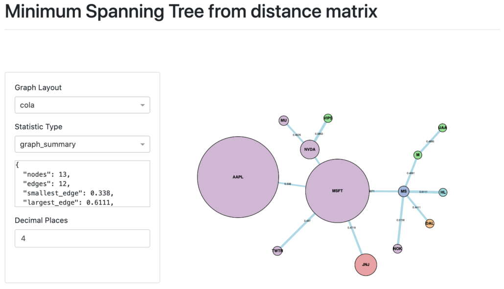
Given your interest in finance, consider the problem of analyzing relationships between stocks. We can model stocks as vertices in a graph and the "distance" between them based on how correlated their price movements are. An MST of this graph would reveal the most essential connections, highlighting clusters of stocks that move together. This is not just a theoretical exercise; it's a technique used in computational finance to understand market structure.

An MST connecting various stock tickers. The edges represent a "distance" based on correlation, and the tree structure reveals core relationships within this set of assets. For instance, you can see a tech-centric cluster around MSFT and AAPL.

What is a Minimum Spanning Tree?

Before we can find the minimum spanning tree, let's first define what a spanning tree is. For a given connected, undirected graph, a spanning tree is a subgraph that meets two conditions:

It includes all the vertices of the original graph.
It is a tree, meaning it is connected and has no cycles. This implies it uses the minimum possible number of edges to connect all vertices, which is exactly $V - 1$ edges, where $V$ is the number of vertices.

Now, let's add weights. In a weighted graph, each edge has a cost. The cost of a spanning tree is the sum of the weights of all its edges. A graph can have many different spanning trees, each with a potentially different total cost. The Minimum Spanning Tree (MST) is a spanning tree with the lowest possible total cost.

[PDF] Greedy algorithms1 1 Minimum spanning trees - People @EECS

This document from UC Berkeley's CS department provides a concise introduction to the MST problem.

Please read from the beginning of the document up to the start of the section "1.1 A greedy approach". Pay attention to the definition of the problem and the key insight that an optimal solution cannot contain a cycle.

The Central Idea: A "Safe" Greedy Choice

MST algorithms are classic examples of greedy algorithms. At each step, they make a choice that looks best at the moment. For MSTs, this means repeatedly adding the "best" available edge to our growing tree. But what constitutes the "best" edge? And how do we know that adding it won't prevent us from finding the optimal solution later?

We need to identify a rule for picking a "safe edge"—an edge that is guaranteed to be part of at least one MST. If we can find such a rule and apply it $V - 1$ times, we will have successfully built an MST. This brings us to the core principle that justifies the greedy approach for all MST algorithms: the Cut Property.

The Cut Property

Let's first define two terms:

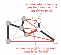
A cut is a partition of the vertices of a graph into two non-empty, disjoint sets. Think of it as drawing a line that divides all vertices into two groups.
A crossing edge is an edge that connects a vertex from one set to a vertex from the other set.

This image illustrates a cut. The vertices are partitioned into a gray set and a white set. The red edges are "crossing edges" because they connect a gray vertex to a white vertex. The Cut Property focuses on the lightest of these red edges.

The Cut Property states:

For any cut in a graph, the minimum-weight edge that crosses the cut is a safe edge (i.e., it must be part of some MST).

This is a powerful statement. It means that no matter how we partition the vertices, we can always find at least one edge that we can safely add to our MST.

To build a strong intuition for this property, let's watch a video that explains it visually and provides a clear proof by contradiction.

vid5 the cut property

This video by Josh Hug from UC Berkeley offers an excellent and concise explanation of the Cut Property.

Please watch from the beginning to the end of the proof. Focus on: The definitions of a cut and a crossing edge. The statement of the property and the example provided. The key takeaway is its surprising generality—it works for any arbitrary cut. The proof by contradiction. This is the logical justification for why the property holds. The argument shows that if we assume the minimum crossing edge isn't in the MST, we can always create a better (or equally good) spanning tree by swapping it in.

For a more formal reinforcement of this concept, you can review the proof in the following document.

[PDF] Minimum Spanning Trees - Bowdoin College

These lecture notes provide a formal proof of the Cut Theorem (another name for the Cut Property).

Read the section titled "The cut theorem". This text formalizes the argument you saw in the video. The core idea is the "exchange argument": if an MST T does not contain the lightest crossing edge e, you can add e to T (creating a cycle) and remove another, heavier crossing edge (x, y) from that cycle to form a new, cheaper spanning tree T'. This contradicts the assumption that T was an MST.

Two Strategies, One Principle: Prim's and Kruskal's

The Cut Property provides a generic template for any greedy MST algorithm:

Start with an empty set of edges.
While we don't have $V - 1$ edges yet:
a. Find some cut that doesn't split any of the edges we've already picked.
b. Find the minimum-weight edge crossing that cut.
c. Add that edge to our set.

The two most famous MST algorithms, Prim's and Kruskal's, are simply two different and clever ways of applying this template.

Intuition Behind Prim's Algorithm

Prim's algorithm grows a single tree from a starting vertex. At every step, the set of edges chosen always forms one connected component (a single tree).

The Greedy Choice: Find the cheapest edge that connects a vertex inside the current tree to a vertex outside the tree.
How it uses the Cut Property: The cut is defined by the vertices already in the tree (let's call this set S) and all other vertices (V-S). Prim's algorithm, by definition, finds the minimum-weight edge crossing this specific (S, V-S) cut and adds it to the tree. The Cut Property guarantees this choice is safe. The algorithm then grows S by one vertex and repeats the process.

Intuition Behind Kruskal's Algorithm

Kruskal's algorithm takes a different approach. It starts with each vertex as its own tiny island (a forest of V trees) and progressively merges them by adding edges.

The Greedy Choice: Consider all edges in the entire graph, sorted by weight from smallest to largest. Add the next edge in the list, but only if it does not form a cycle with the edges already chosen.
How it uses the Cut Property: When Kruskal's considers adding an edge (u, v), the vertices u and v must belong to two different components (or "islands") in the forest. If they were in the same component, adding the edge would create a cycle. Let's say u is in component $C_{u}$ . We can define a cut as $(C_{u}, V - C_{u})$ . Because the algorithm processes edges in increasing order of weight, the edge (u, v) is the absolute lightest edge that connects a vertex in $C_{u}$ to a vertex outside $C_{u}$ . Therefore, by the Cut Property, (u, v) is a safe edge.

This short reading summarizes how both algorithms are instantiations of the same general principle.

[PDF] Minimum Spanning Trees - Bowdoin College

This section of the lecture notes concisely explains how both Prim's and Kruskal's algorithms are justified by the cut theorem.

Read the text at the end of section 5. This directly connects the strategy of each algorithm to a specific choice of cut, solidifying the intuition.

To see a high-level visual of how these two strategies play out, you can watch the following segments. Don't worry about the implementation details; just focus on the overall process.

3.5 Prims and Kruskals Algorithms - Greedy Method

This video by Abdul Bari illustrates the step-by-step execution of both algorithms.

Watch the demonstration of Prim's algorithm from this example. Notice how it always maintains a single connected tree, expanding it one edge at a time. Next, watch the demonstration of Kruskal's algorithm from this example. Observe how it picks the cheapest edges globally, creating a "forest" of components that eventually merge into a single tree.

Conclusion

In this lesson, we laid the conceptual groundwork for understanding Minimum Spanning Tree algorithms. We moved from the problem of finding the shortest path to that of finding the cheapest network to connect all nodes.

Key Takeaways:

A Minimum Spanning Tree (MST) is the lowest-cost subgraph that connects all vertices in a weighted, undirected graph without forming any cycles.
The correctness of greedy MST algorithms is guaranteed by the Cut Property, which states that for any partition of vertices into two sets, the minimum-weight edge crossing the partition is part of some MST.
Prim's algorithm applies this property by growing a single tree. The cut is between the vertices in the tree and those outside.
Kruskal's algorithm applies this property by merging a forest of components. The cut is between the component of one endpoint and all other vertices.

We now understand why these greedy strategies work. In our next lesson, we will put this theory into practice and implement Prim's algorithm using a priority queue, seeing its close resemblance to Dijkstra's algorithm. Following that, we'll implement Kruskal's algorithm, where you'll see a fantastic application of the Union-Find data structure you studied earlier.