Dijkstra's Algorithm with Min-Heap

Welcome to the second lesson in our graph algorithms module. In our previous session, you learned how to represent graphs using an adjacency list, a crucial first step for nearly all graph-based tasks. We saw how this representation is both memory-efficient and ideal for traversal algorithms.

Today, we will build directly on that foundation to tackle one of the most famous and useful graph algorithms: Dijkstra's algorithm. The learning outcome for this lesson is to implement Dijkstra's algorithm for single-source shortest paths using a min-heap. This algorithm is a cornerstone of computer science, used in everything from network routing to GPS navigation, and is a frequent topic in coding interviews. We will focus on understanding its greedy logic and mastering the standard, efficient implementation pattern.

The Problem: Shortest Paths in a Weighted Graph

Imagine a road map where cities are nodes and roads are edges, each labeled with the distance (the weight). If you want to find the shortest route from your home city to every other city, how would you do it?

In an unweighted graph, where every edge has the same cost (e.g., 1), a simple Breadth-First Search (BFS) would suffice. BFS explores layer by layer, guaranteeing that it finds the path with the fewest edges. However, in a weighted graph, the path with the fewest edges is not always the shortest one. A direct flight might cost more than a route with two layovers.

Dijkstra's algorithm solves this exact problem for graphs with non-negative edge weights. It's a greedy algorithm that systematically finds the shortest path from a single source node to all other nodes in the graph.

The core idea is beautifully simple:

1. Maintain a set of "visited" nodes for which we have already found the absolute shortest path.
2. At each step, greedily select the "unvisited" node that is closest to the source node based on our current knowledge.
3. Add this node to our "visited" set and update the distances to its neighbors if we find a shorter path through it.

This process is explained very clearly with a travel-cost analogy in the following article from Interview Cake.

The Key to Efficiency: The Min-Heap

In the example you just read, at each step, we needed to find the city with the minimum cost among all unvisited cities. How can we do this efficiently?

• We could scan through our entire list of costs at each step, but that would be slow, leading to an O(V²) algorithm, where V is the number of vertices.
• A much better approach is to use a min-priority queue, which is typically implemented with a min-heap.

A min-heap is a data structure that allows us to:

• Add a new element in O(log N) time.
• Find and remove the minimum element in O(log N) time.

By storing (cost, node) pairs in a min-heap, we can instantly retrieve the node with the current shortest path estimate in logarithmic time. This is the crucial optimization that makes Dijkstra's algorithm efficient for the sparse graphs you'll encounter in interviews. In Python, the heapq module provides a min-heap implementation out of the box.

Algorithm Walkthrough with Animation

Before we dive into the code, let's watch a detailed, animated walkthrough. This will help solidify your intuition for how the distance estimates and the min-heap evolve as the algorithm runs.

The Implementation Pattern

Now that we have the conceptual and visual understanding, let's translate it into a robust Python implementation. We'll use a distances array to store the shortest path costs, an adjacency list to represent the graph (as learned in the last lesson), and Python's heapq module for our min-heap.

The following article provides a complete, well-commented solution that serves as an excellent template.

Let's synthesize what you've just read into a complete, documented function.

import heapq
from collections import defaultdict

def dijkstra(n, edges, src):
    """
    Implements Dijkstra's algorithm to find the shortest paths from a source node
    to all other nodes in a weighted graph.

    Args:
        n (int): The number of nodes in the graph, labeled 0 to n-1.
        edges (List[List[int]]): A list of edges, where each edge is [u, v, weight].
        src (int): The source node.

    Returns:
        Dict[int, int]: A dictionary mapping each reachable node to its shortest
                        path distance from the source. Unreachable nodes are excluded.
    """
    # 1. Build adjacency list
    adj = defaultdict(list)
    for u, v, w in edges:
        adj[u].append((v, w))

    # 2. Initialize distances and the min-heap
    distances = {}  # Using a dict to store final shortest paths
    min_heap = [(0, src)]  # (distance, node)

    # 3. Main loop
    while min_heap:
        # Pop the node with the smallest distance from the heap
        dist, node = heapq.heappop(min_heap)

        # IMPORTANT: Stale entry check
        # If we have already found a shorter path to this node, skip.
        if node in distances:
            continue
        
        # Lock in the shortest path for this node
        distances[node] = dist

        # 4. Relax edges for all neighbors
        for neighbor, weight in adj[node]:
            if neighbor not in distances:
                new_dist = dist + weight
                heapq.heappush(min_heap, (new_dist, neighbor))
    
    return distances

The image below provides another excellent visualization of this process. It shows the graph, the state of the priority queue at each step (with stale entries crossed out), and the final cost (our distances dictionary) and pred (predecessor) table.

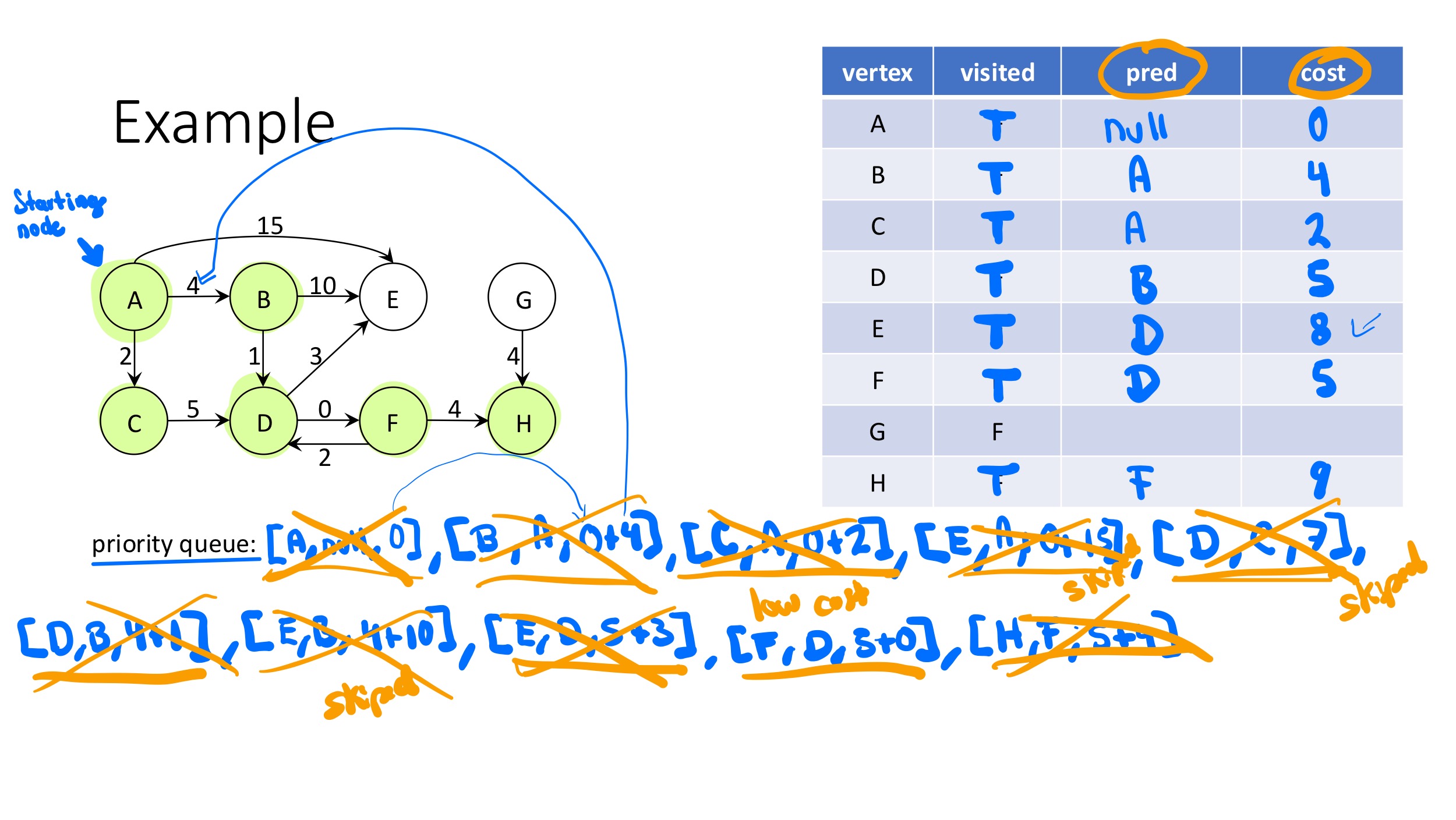
An illustration of Dijkstra's algorithm in action. The table on the right tracks the final cost and pred (predecessor) for each node. The list at the bottom shows the state of the priority queue, with crossed-out entries representing "stale" paths that were superseded by shorter ones.

Complexity Analysis

Understanding the performance of this algorithm is critical for interviews. The use of a min-heap is what makes it so efficient.

• Time Complexity: O((E + V) log V), where V is the number of vertices and E is the number of edges.

  • We build the adjacency list in O(E) time.
  • The main while loop runs until every reachable vertex is processed once. In the worst case, we might process all V vertices. Each heappop operation takes O(log V) time. This gives us O(V log V).
  • For every edge, we might perform one heappush operation, which also takes O(log V). This gives us O(E log V).
  • Combining these, the dominant complexity is O(V log V + E log V), which is often simplified to O(E log V) for connected graphs where E is at least V-1.

• Space Complexity: O(V + E).

  • The adjacency list requires O(V + E) space.
  • The distances dictionary can store up to V entries.
  • The min_heap in the worst case can store an entry for each edge, so O(E) space.
  • Therefore, the total space is dominated by the adjacency list and the heap.

The Code and Debug article you read earlier also has a concise complexity analysis section you can refer back to.

Conclusion

In this lesson, we dissected Dijkstra's algorithm, a fundamental tool for solving shortest path problems. We moved from the high-level greedy concept to a practical, efficient implementation ready for coding challenges.

Key Takeaways:

• Dijkstra's algorithm finds the single-source shortest paths in a weighted graph with non-negative edges.
• It operates on a greedy principle: always explore the unvisited node with the smallest known distance from the source.
• A min-heap (priority queue) is the essential data structure for an efficient implementation, allowing quick retrieval of the next node to visit. Its use reduces the time complexity from O(V²) to O(E log V).
• The core implementation pattern involves a distances structure, a min-heap storing (cost, node) tuples, and a loop that pops the minimum element and relaxes its neighbors.
• Handling stale entries in the heap by checking if a node has already been finalized is a crucial detail for a correct and efficient implementation.

In our next lesson, we will apply this powerful algorithm to various problems, including those on implicit graphs like grids, to see how versatile this pattern truly is.