Diminishing Returns in Short-Run Production

Introduction

Welcome to our third lesson on the costs of production. In the previous lesson, we mapped out a firm's production capabilities in the short run by calculating and graphing the total product (TP), marginal product (MP), and average product (AP) of labor. We observed that the marginal product curve typically rises at first, reaches a peak, and then declines.

Today, we will explore the fundamental economic principle that explains this pattern: the law of diminishing marginal returns. Your learning outcome for this lesson is to explain this law in the context of short-run production. We will answer the crucial question: why does the productivity of each additional worker eventually fall? Understanding this law is not just key to production theory; as we will see, it forms the bedrock for understanding a firm's costs.

1. Defining the Law

First, let's establish a clear definition. The law of diminishing marginal returns is a short-run phenomenon. It states that as you add more and more units of a variable input (like labor) to a fixed amount of other inputs (like capital and land), the marginal product of the variable input will eventually decrease.

It's crucial to note the word "eventually." As we saw last lesson, marginal product can increase at first. It's also important to distinguish "diminishing" from "negative." When returns are diminishing, total output is still increasing, but at a slower rate.

To start, let's watch a short video that introduces the concept and its context.

2. The "Why": Increasing vs. Diminishing Returns

Now that we have a formal definition, let's explore why this law holds. The behavior of the marginal product curve can be broken down into distinct stages.

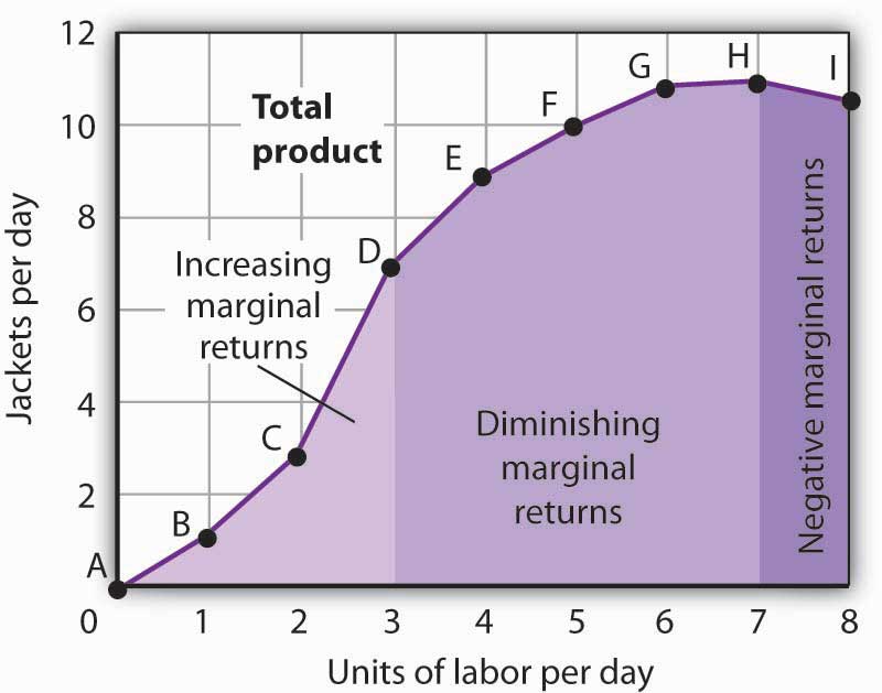
1. Increasing Marginal Returns: Initially, as the first few workers are hired, they can specialize in tasks. With a fixed amount of capital (e.g., machinery, workspace), there might be more than enough equipment to go around. One worker might struggle to operate three machines, but three workers can each take one machine and coordinate their efforts. This specialization and better utilization of fixed capital leads to a rising marginal product—each new worker adds more to total output than the one before.

2. Diminishing Marginal Returns: After a certain point, the benefits of specialization are exhausted, and the fixed capital becomes a constraint. Imagine a busy kitchen with a fixed number of stoves and prep stations. As you add more chefs, they start to get in each other's way. They have to wait to use the stove or find an open counter. The fixed inputs become "crowded." While each new chef still increases the total number of meals produced (total product rises), their individual contribution (marginal product) is smaller than the chef hired before them. This is the stage of diminishing marginal returns.

3. Negative Marginal Returns: If the firm continues to hire workers, the workspace can become so overcrowded that adding another worker is actually counterproductive. They might bump into each other, disrupt workflows, and cause total output to fall. At this point, the marginal product becomes negative.

The following video provides a detailed walkthrough of these stages using a numerical example of a pizza business.

3. A Deeper Look at the Stages of Production

To solidify your understanding, let's turn to a text-based explanation that formally outlines these stages and provides a powerful analogy for why diminishing returns are an inevitable law of production.

As the reading explains, these three stages of returns can be mapped directly onto the total product curve you learned about in the last lesson.

4. An Important Distinction: Diminishing Returns vs. Returns to Scale

It is essential to distinguish the law of diminishing marginal returns from a related, but different, long-run concept called "returns to scale."

• Law of Diminishing Marginal Returns (Short Run): Examines what happens to output when we add more of one variable input while holding at least one other input fixed. The eventual decline in MP is due to the fixed input acting as a constraint.
• Returns to Scale (Long Run): Examines what happens to output when we increase all inputs by the same proportion. Since all inputs are variable in the long run, the firm can scale up its entire operation (e.g., build a bigger factory and hire more workers).

We will explore returns to scale later in this module. For now, simply remember that diminishing marginal returns is strictly a short-run concept, defined by the presence of a fixed factor of production.

Conclusion

In this lesson, we have moved beyond simply describing the production curves to explaining the economic logic that shapes them. The law of diminishing marginal returns is a fundamental principle that governs all short-run production processes.

Here are the key takeaways:

• The law states that as a firm adds more of a variable input to a fixed input, the marginal product of the variable input will eventually decline.
• This pattern is explained by two forces: initially, specialization and better use of fixed capital cause increasing returns.
• Eventually, the fixed input becomes a constraint, leading to crowding and diminishing returns.
• It is critical to distinguish diminishing returns (where MP is positive but falling) from negative returns (where MP is negative and TP is falling).
• This law applies only in the short run, where at least one factor of production is fixed.

You now have a solid understanding of a firm's production behavior. In our next lesson, we will see how this behavior directly translates into a firm's costs. The shape of the marginal product curve you've analyzed today is a mirror image of the marginal cost curve we will derive next. This connection is one of the most elegant and important relationships in microeconomics.