Permutations with Backtracking

Welcome to our next lesson on backtracking! In our previous lessons, we focused on problems of selection—choosing subsets and combinations where the order of elements didn't matter. We used a start_index in our recursion to ensure that once we considered an element, we never looked back at previous elements, naturally avoiding duplicates and permutations.

Today, we shift our focus to problems of arrangement. This lesson addresses the learning outcome: Generate all permutations of a list using backtracking with a used-set or by swapping elements. A permutation is a specific ordering of a set of elements. For the set {1, 2, 3}, [1, 2, 3] and [1, 3, 2] are two different permutations. Our goal is to generate every possible unique arrangement. This requires a different backtracking strategy, as we now need to use every element from the input, but only once per arrangement. We will explore two canonical patterns for achieving this.

The Core Idea: Filling Slots

Think of generating a permutation of n elements as filling n empty slots.

• For the first slot, you have n choices.
• Once you've placed an element in the first slot, you have n-1 remaining choices for the second slot.
• This continues until you have only one choice left for the final slot.

This sequence of choices gives a total of n * (n-1) * ... * 1 = n! possible permutations. This "choose from what's available" structure is a perfect fit for a backtracking algorithm, where each level of recursion corresponds to filling the next slot in our permutation. The main challenge becomes: how do we keep track of which elements are "available" at each step?

Approach 1: Backtracking with a used Array

The most straightforward way to track available elements is to use an auxiliary data structure. A boolean array, often called used or visited, is a common choice. This array will be the same size as the input nums, and used[i] will be true if nums[i] is already part of the permutation we are currently building.

The recursive function will build the permutation step by step. At each level of the recursion, it will iterate through the entire original nums array and try to place an unused element into the current slot.

The AlgoMonster article on "Permutations" provides a clear, step-by-step guide to this approach. It walks through the intuition, algorithm, and a detailed example.

The core logic of this used array method is:

1. Base Case: If the permutation we are building (current_permutation) has the same length as the input nums, we have found a valid permutation. Add a copy of it to our results and return.
2. Recursive Step: Loop through all numbers in the original nums array from index j = 0 to n-1.
3. Choice: If nums[j] has not been used yet (!used[j]):
   • Add nums[j] to current_permutation.
   • Mark it as used: used[j] = true.
   • Recursively call the function to fill the next slot.
   • Backtrack: Remove nums[j] from current_permutation (or simply overwrite it in the next loop iteration if using a fixed-size array for the path) and unmark it: used[j] = false. This is crucial, as it makes nums[j] available for other branches of the recursion.

This method is highly intuitive because it directly models the "fill the slots" idea while explicitly managing which elements are available. Its main trade-off is the O(n) extra space required for the used array and the current_permutation list.

Approach 2: Backtracking with In-Place Swapping

An alternative, more space-efficient approach eliminates the need for an explicit used array. Instead, it cleverly uses the input array itself to track which elements are available by performing in-place swaps.

The core idea is to maintain an invariant: at any recursive call backtrack(index), the elements from nums[0] to nums[index - 1] are considered "fixed" for the current permutation path. The elements from nums[index] to nums[n - 1] are the "available" elements for the remaining slots.

To decide which element to place at index, we iterate from j = index to n-1 and swap nums[index] with nums[j]. This brings each available element into the index position one by one. After each recursive call, we swap back to restore the array for the next iteration of the loop.

This video from "take U forward" provides an excellent visualization of this swapping mechanism.

Let's visualize this with the provided image for [1, 2, 3].

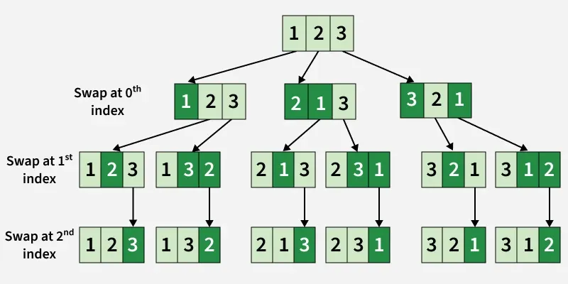
Let's trace the leftmost branch:

1. backtrack(index=0):
   • i=0: Swap nums[0] with nums[0] (no change). nums is [1, 2, 3]. 1 is now fixed at index 0.
   • Call backtrack(index=1).
2. backtrack(index=1):
   • i=1: Swap nums[1] with nums[1] (no change). nums is [1, 2, 3]. 2 is now fixed at index 1.
   • Call backtrack(index=2).
3. backtrack(index=2):
   • i=2: Swap nums[2] with nums[2] (no change). nums is [1, 2, 3]. 3 is now fixed at index 2.
   • Call backtrack(index=3).
4. backtrack(index=3):
   • Base case index == 3. Add [1, 2, 3] to results. Return.
5. Back in backtrack(index=2), the loop finishes. We swap nums[2] and nums[2] back (no change). Return.
6. Back in backtrack(index=1), the i=1 iteration is done.
   • i=2: Swap nums[1] with nums[2]. nums becomes [1, 3, 2]. 3 is now fixed at index 1.
   • Call backtrack(index=2). This will eventually add [1, 3, 2] to the results.
   • After the call returns, swap back: nums becomes [1, 2, 3] again.

This in-place modification is elegant and saves space, as you only need the recursion stack, which is O(n) depth. Both methods have a time complexity of O(n * n!) because we generate n! permutations, and copying each to the result list takes O(n) time.

Handling Duplicates: A Preview

Both methods we've discussed assume the input array contains distinct elements. What if the input were [1, 2, 2]? The algorithms as-is would produce duplicate permutations in the output (e.g., [2, 1, 2] would be generated twice).

The image above hints at the challenge. Simply using a visited array isn't enough. We need an additional rule to avoid starting a new search path with a duplicate number if we've already explored a path starting with that same number at this level of recursion. This is a classic follow-up problem (like LeetCode's "Permutations II").

This is precisely what we will tackle in our next lesson: adapting these permutation templates to gracefully handle duplicates and produce a set of unique permutations.

Conclusion

In this lesson, we transitioned from combination problems to permutation problems, where element order is paramount. You've learned the two primary backtracking patterns for generating all permutations of a set of distinct elements.

Key Takeaways:

• Permutations vs. Combinations: For permutations, we can't just use a start_index to move forward. We must be able to select from all available elements at each step.
• Approach 1: used Array: An intuitive method that uses an O(n) boolean array to explicitly track which elements have been placed in the current permutation path.
• Approach 2: In-place Swapping: A more space-efficient O(1) space (excluding recursion stack) method that cleverly partitions the array into "fixed" and "available" parts by swapping elements.
• Backtracking is Key: In both methods, the "undo" step (un-marking an element as used, or swapping back) is what enables the algorithm to explore all possible branches of the decision tree.

In our next lesson, we will build directly on these patterns. We will introduce a small but critical modification to our logic that will allow us to handle inputs with duplicate numbers and ensure our output contains only unique permutations.