Backtracking for Subsets

Welcome back! In our previous lesson, we established the conceptual foundation of backtracking, framing it as a recursive search strategy guided by choices, constraints, and a goal. We saw how this "choose, explore, un-choose" pattern allows for a systematic exploration of a problem's solution space, much like a depth-first search on an implicit decision tree.

Today, we'll put that theory into practice. Our goal is to generate all subsets of a set using a backtracking template. This is a classic, foundational problem that perfectly illustrates the backtracking framework in its purest form. By mastering this pattern, you'll gain a solid blueprint that can be adapted to solve a wide variety of combinatorial problems.

Framing the Subsets Problem

First, let's define the problem. Given a set of unique numbers, like [1, 2, 3], we want to generate its power set—the set of all possible subsets. For [1, 2, 3], this would include the empty set [], single-element sets like [1], two-element sets like [1, 2], and the full set [1, 2, 3].

How does this fit the backtracking framework we learned?

1. Choice: For each element in the input array, we face a simple binary decision: do we include it in the subset we are currently building, or do we exclude it?
2. Constraints: In this basic version of the problem (with unique elements), there are no constraints. Every choice is valid. We are free to explore all possibilities without restriction.
3. Goal: We have reached our goal when we have made a decision (either include or exclude) for every single element in the original array. At that point, the subset we have constructed is complete, and we should add it to our list of solutions.

The AlgoMonster article on this problem provides an excellent explanation of this core intuition.

Visualizing the Decision Tree

This series of binary choices creates a decision tree. Starting with an empty subset, we consider the first element. This decision creates two branches: one where we include the element and one where we don't. From each of those branches, we consider the second element, again creating two new branches for each.

This process continues until all elements have been considered. Each path from the root of the tree to a leaf node represents one unique subset.

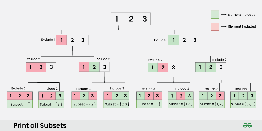
This "Pick / Not Pick" pattern is a fundamental backtracking strategy. The visual cheat sheet below shows how it compares to other common patterns we'll explore later.

The Backtracking Algorithm

Now, let's translate this decision tree into a recursive algorithm. We'll design a helper function that performs a depth-first search on this tree.

Let's consolidate those ideas into a concrete template:

1. Define a recursive helper function, let's call it backtrack(index, current_subset).

   • index: The index of the element in the input array we are currently making a decision about.
   • current_subset: The list representing the subset we are building along the current path.

2. Base Case (The Goal): If index has gone past the end of the array, it means we have made a decision for every element.

   • Add a copy of current_subset to our final results list.
   • Return to the previous recursive call.

3. Recursive Step (The Choices):

   • Decision 1: Exclude nums[index]. To explore this branch, we do nothing to current_subset and simply make a recursive call for the next element: backtrack(index + 1, current_subset).
   • Decision 2: Include nums[index]. This involves the full "choose, explore, un-choose" cycle:
     • Choose: Add nums[index] to current_subset.
     • Explore: Make a recursive call: backtrack(index + 1, current_subset).
     • Un-choose (Backtrack): Remove nums[index] from current_subset. This step is vital. It reverts the state of current_subset so that other branches of the recursion are not affected by this choice.

This video from NeetCode provides a fantastic walkthrough of this logic, connecting the decision tree directly to the code implementation.

Implementation and Common Pitfalls

With the logic clear, let's look at a complete implementation. Since you're familiar with LeetCode, you'll recognize this style.

def subsets(nums):
    result = []
    current_subset = []

    def backtrack(index):



        # Base Case: all decisions made, add the constructed subset
        if index >= len(nums):



            # IMPORTANT: Add a copy, not a reference
            result.append(list(current_subset))
            return




        # Decision 1: Exclude the element nums[index]
        # Move on to the next decision without adding to the subset
        backtrack(index + 1)




        # Decision 2: Include the element nums[index]
        # Choose
        current_subset.append(nums[index])



        # Explore
        backtrack(index + 1)



        # Un-choose (Backtrack)
        current_subset.pop()

    backtrack(0)
    return result




# Example:
print(subsets([1, 2, 3]))



# Output: [[], [3], [2], [2, 3], [1], [1, 3], [1, 2], [1, 2, 3]]
# Note: The order of subsets in the output may vary depending on
# the order of the include/exclude recursive calls.

This implementation follows a slightly different, but equivalent, order of operations than the one described in the AlgoMonster text. Here, the exclude call is made first, followed by the include block. The result is the same. The key is that both branches are explored.

There are two very common mistakes when implementing this pattern, both of which are critical to understand for practical coding.

Complexity Analysis

Finally, let's analyze the performance of our algorithm. Given your CS background, you'll recognize the exponential nature of this problem.

• Time Complexity: $O(n\cdot 2^n)$.

  • We generate $2^n$ subsets in total.
  • For each subset, when we reach the base case, we create a copy. In the worst case, a subset can have $n$ elements, so copying it takes $O(n)$ time.
  • This gives us a total time complexity of $n\times 2^n$.

• Space Complexity: $O(n)$.

  • This refers to the auxiliary space used by the algorithm, not including the space required to store the final output.
  • The depth of our recursion is at most $n$, so the call stack uses $O(n)$ space.
  • The current_subset list also stores at most $n$ elements.
  • Therefore, the space complexity is dominated by the recursion depth, resulting in $O(n)$.

Conclusion

In this lesson, you've successfully translated the abstract backtracking framework into a concrete, working algorithm. You saw how the "subsets" problem can be elegantly solved by modeling it as a series of binary "include/exclude" decisions, which naturally maps to a recursive DFS traversal of a decision tree.

Key Takeaways:

• Subset Generation Pattern: For each element, make two recursive calls: one representing its exclusion and one representing its inclusion.
• Backtracking is Key: The "un-choose" step (e.g., current_subset.pop()) is essential to revert the state after exploring a path, ensuring that decisions do not interfere across different branches of the decision tree.
• Copy on Save: When a solution is found (at the base case), you must save a copy of the current state, not a reference to it, as the state object will continue to be modified.
• Complexity: Generating all $2^n$ subsets inherently requires exponential time, specifically $O(n\cdot 2^n)$ due to the copying of results.

In our next lesson, we will build directly on this template. We'll introduce a new challenge: how to handle duplicate elements in the input array and modify our logic to avoid generating duplicate subsets in the output. This will require us to start thinking about the "constraints" pillar of backtracking more actively.