GKP Codes: Structure and Error Correction in Phase Space

Hello! Welcome to our next lesson in the series on recent advances in quantum error correction.

In our last lesson, we explored Schrödinger cat codes, which encode a qubit into a superposition of coherent states. We saw that their structure is tailored to combat "subtractive" errors like single photon loss, which is detected by a change in the state's photon number parity.

Today, we shift our focus to a different, yet equally important, family of bosonic codes: the Gottesman-Kitaev-Preskill (GKP) codes. As you'll see, these codes have a completely different structure in phase space, making them naturally suited to correcting "additive" errors in the form of small, random displacements. This lesson directly addresses the learning outcome: Analyze the structure of Gottesman-Kitaev-Preskill (GKP) codes in phase space and derive their mechanism for correcting small displacement errors.

1. The Structure of GKP States

While cat codes are superpositions of a few (2 or 4) coherent states, GKP states are superpositions of an infinite number of states, forming a regular grid or lattice in phase space. Let's start with a high-level visual and auditory introduction.

As the video illustrates, the GKP state has a unique and intricate structure. To understand it formally, we will dive into a more detailed resource.

Let's break down the key concepts from that reading.

Ideal GKP Codes

The ideal GKP code is defined within the Hilbert space of a single harmonic oscillator. Its core properties are:

• Stabilizers: The logical subspace is defined as the simultaneous +1 eigenspace of two commuting stabilizer operators. For a square lattice GKP code, these are displacement operators:

  $${\hat{S}}_q=\hat{X}(2\sqrt{\pi })=e^{-i2\sqrt{\pi }\hat{p}}$$ $${\hat{S}}_p=\hat{Z}(2\sqrt{\pi })=e^{i2\sqrt{\pi }\hat{q}}$$

  Since $[\hat{q},\hat{p}]=i$, these operators commute, $[{\hat{S}}_q,{\hat{S}}_p]=0$, allowing for simultaneous stabilization. This should feel familiar from the stabilizer codes you studied in Module 5.

• Logical States: The logical basis states can be expressed as superpositions of position eigenstates $|q⟩$. They form an infinite "comb" of Dirac delta functions:

  $$|0_L⟩\propto \sum _{j=-\infty }^{\infty }|q=2j\sqrt{\pi }⟩$$ $$|1_L⟩\propto \sum _{j=-\infty }^{\infty }|q=(2j+1)\sqrt{\pi }⟩$$

  The state $|0_L⟩$ consists of peaks at even integer multiples of $\sqrt{\pi }$, while $|1_L⟩$ has peaks at odd integer multiples.

In phase space, the Wigner function of an ideal GKP state like $|0_L⟩$ is a 2D grid of delta functions.

Finite-Energy GKP Codes

Ideal GKP states are unphysical as they contain infinite energy. To create a physically realizable version, we apply a Gaussian "envelope" operator ${\hat{E}}_{\Delta }=\exp (-{\Delta }^2{\hat{a}}^{†}\hat{a})$ to the ideal states. This has two effects:

1. Each delta-function peak in phase space is broadened into a small Gaussian peak of width $\sim \Delta$.
2. The entire infinite grid is enveloped by a larger Gaussian of width $\sim 1/\Delta$.

The parameter $\Delta$ represents a trade-off:

• Small $\Delta$: The state is closer to ideal, with well-defined, narrow peaks. This provides better error correction capabilities but requires higher energy (squeezing), making it harder to prepare and maintain.
• Large $\Delta$: The state has lower energy but the peaks are broader and overlap more, reducing the code's ability to correct errors.

The Wigner functions for the finite-energy GKP logical states, shown in Figure 2-5 of the thesis, provide an excellent visualization of this structure. The logical $|0_L⟩$ and $|1_L⟩$ (or $|\pm Z_L⟩$) states have grids offset along the $q$ axis, while the logical $|\pm X_L⟩$ states are grids offset along the $p$ axis.

2. The GKP Error Correction Mechanism

GKP codes are designed to correct the primary error affecting continuous-variable systems: small, unknown displacements in phase space. This error channel maps a state $\rho$ to $\hat{D}(\delta \alpha )\rho {\hat{D}}^{†}(\delta \alpha )$, where $\delta \alpha =(\delta q+i\delta p)/\sqrt{2}$ is a small, random complex number.

The Correction Principle

The fundamental idea is that because the GKP state is periodic in phase space, we only need to know an error's value modulo the lattice spacing to correct it.

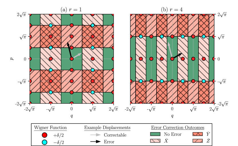
As shown in the figure above, phase space is tiled into cells centered on the lattice points.

• If a displacement error is small enough (e.g., $|\delta q|,|\delta p|<\sqrt{\pi }/2$), the state remains within its original cell. We can measure the displacement $(\delta q,\delta p)$ and apply a correcting displacement $\hat{D}(-\delta \alpha )$ to move the state back to the center of the cell.
• If the displacement is too large (e.g., $|\delta q|>\sqrt{\pi }/2$), the state is pushed into a neighboring cell. Our measurement will now identify the center of this new cell as the target. Correcting to this new center is equivalent to a perfect correction followed by a logical operator (${\hat{X}}_L$ or ${\hat{Z}}_L$), resulting in a logical error.

To formalize this, we can define distinct zones in phase space.

Deriving the Mechanism with an Ancilla

As the paper explains, measuring the stabilizers ${\hat{S}}_q$ and ${\hat{S}}_p$ is not a simple projective measurement. Instead, it is implemented by coupling the GKP oscillator (the data qubit) to another GKP oscillator (the ancilla) and then measuring the ancilla. The circuit in Figure 2 of arXiv:2308.01549v1 uses a SUM gate, ${\hat{U}}_{\text{SUM}}=e^{-i{\hat{q}}_1{\hat{p}}_2}$, to achieve this.

Let's trace the effect of a displacement error $u_1$ on the data qubit's position quadrature.

1. Ideal Ancilla Case:

• The data qubit has an initial displacement error $u_1$. The ancilla is a perfect GKP $|+⟩$ state with no error ($u_2=0$).
• After the SUM gate, the ancilla's position quadrature becomes $q_2^{\prime }=q_2+q_1$. An ideal GKP $|+⟩$ state has position peaks at $k\sqrt{\pi }$. A measurement of the ancilla's position will therefore yield an outcome $q_{meas}=k\sqrt{\pi }+u_1$.
• To infer the error, we find the nearest lattice point: $g(q_{meas})=q_{meas}(\mathrm{mod}\sqrt{\pi })$. With a high probability for small $u_1$, our guess for the error is $u_1$.
• We apply a correction displacement of $-g(q_{meas})$ to the data qubit. The residual displacement is $u^{\prime }=u_1-g(u_1)$.
• As derived in the paper (Eq. 30), this residual error $u^{\prime }$ is discrete:
  • If $u_1$ is in the NPZ (e.g., $|u_1|<\sqrt{\pi }/2$), then $u^{\prime }=0$ (modulo $2\sqrt{\pi }$). Perfect correction.
  • If $u_1$ is in the PZ (e.g., $\sqrt{\pi }/2<u_1<3\sqrt{\pi }/2$), then $u^{\prime }=\sqrt{\pi }$ (modulo $2\sqrt{\pi }$). This is a logical Pauli-${\hat{X}}_L$ error.

2. Physical Ancilla Case (The Realistic Scenario):
This is the crucial part. The ancilla is also a physical GKP state and has its own small displacement error, $u_2$.

• The measurement outcome of the ancilla's position is now $q_{meas}=k\sqrt{\pi }+u_1+u_2$.
• Our inferred error is $g(q_{meas})=g(u_1+u_2)$.
• The residual displacement on the data qubit is now $u^{\prime }=u_1-g(u_1+u_2)$.
• As shown in Eq. (36), if $u_1+u_2$ falls into a cell centered at $k\sqrt{\pi }$, the residual error becomes $u^{\prime }=u_1-(u_1+u_2-k\sqrt{\pi })=k\sqrt{\pi }-u_2$.

This is a profound result. The error correction process effectively substitutes the unknown error of the data qubit ($u_1$) with the unknown error of the ancilla qubit ($-u_2$), while re-centering it on the GKP grid. This is why high-quality ancillas (small $u_2$, i.e., small $\tilde{\Delta }$ in the paper's notation) are essential for effective GKP error correction. The distribution of this continuous residual error, shown in Figure 5 of the paper, clearly illustrates that a better ancilla (smaller $\tilde{\Delta }$) leads to a sharper peak around $u^{\prime }=0$, meaning a more successful correction.

Conclusion

In this lesson, we have analyzed the Gottesman-Kitaev-Preskill code, a cornerstone of bosonic quantum error correction.

Key Takeaways:

• Structure: GKP codes encode a qubit into a periodic grid-like structure in the phase space of a harmonic oscillator. Ideal states are infinite-energy "combs" of delta functions, while physical states are finite-energy versions with Gaussian-broadened peaks.
• Error Model: They are designed to correct small, additive displacement errors, which are common in continuous-variable systems.
• Correction Mechanism: The correction works by measuring the oscillator's position and momentum quadratures modulo the lattice period. This is typically done by coupling the oscillator to an ancilla GKP state.
• Ancilla's Role: The process effectively transfers the error from the data qubit to the ancilla. A perfect correction relies on a perfect ancilla; a physical ancilla replaces the data error with its own error, limiting the overall fidelity.

Preview of the next lesson:
Both cat codes and GKP codes are examples of active quantum error correction (QEC), where we detect errors and apply real-time corrections. This is a powerful but demanding approach. For the noisy quantum devices available today, a different strategy is often more practical. In our next lesson, we will explore the principles of quantum error mitigation (QEM). Instead of actively correcting errors, QEM techniques aim to estimate and computationally subtract their effects during data post-processing, providing a pathway to useful results on near-term hardware.