Fundamentals of Dynamic Programming

Welcome to the module on Dynamic Programming! This is often considered one of the most challenging topics in algorithms, but it's also one of the most powerful. My goal is to demystify it for you. We'll build up your understanding from first principles, focusing on a structured way of thinking that you can apply to any problem, which should help manage any "algo phobia."

In previous modules, particularly the one on recursion, you saw how to solve problems by breaking them down into smaller instances of the same problem. Dynamic Programming, or DP, takes this a step further. It's an optimization technique for recursive problems that have a specific characteristic: overlapping subproblems.

In this lesson, you will learn to dissect any dynamic programming problem into four fundamental components. Mastering this framework is the key to turning DP from a source of anxiety into a reliable tool in your problem-solving arsenal.

Your learning outcome for today is to identify the state, transition, base cases, and evaluation order of a dynamic program.

The Problem with Plain Recursion

Let's start with a familiar problem: calculating the Nth Fibonacci number. A naive recursive solution looks something like this:

function fib(n: number): number {
    if (n <= 1) {
        return n;
    }
    return fib(n - 1) + fib(n - 2);
}

This is elegant, but terribly inefficient. To see why, let's trace the calls for fib(4):

As you can see, we compute fib(2) twice from scratch. fib(1) is computed three times. This redundancy is the "overlapping subproblems" property. For larger n, the number of repeated computations explodes, leading to an exponential time complexity, roughly $O(2^n)$. Dynamic programming is all about solving each subproblem just once and storing the result for future use.

A Visual Introduction to the DP Mindset

Before we dive into a formal framework, let's build some intuition. The following video provides a fantastic, animated walkthrough of a classic DP problem—the "climbing stairs" problem. It's very similar to Fibonacci and is a great way to see the core ideas of DP in action.

This video gave you a visual sense of the entire process. Now, let's formalize the concepts you just saw into a reusable framework.

The Four Pillars of a Dynamic Program

Every DP solution, whether top-down or bottom-up, is built on four conceptual pillars. If you can define these four things for any given problem, you can solve it.

1. State: The state is a set of parameters that uniquely defines a subproblem and its solution. It's the "minimum information you need to make a decision." We often use dp[i] or dp[i][j] to store the solution for the state defined by i or (i, j).
2. Transition: The transition is the formula or rule that relates the solution of a given state to the solutions of smaller subproblems. This is also called the recurrence relation.
3. Base Cases: These are the smallest subproblems that can be solved directly, without depending on any other subproblems. They are the starting points for your calculation.
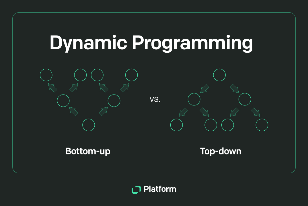
4. Evaluation Order: This is the order in which you solve the subproblems. To calculate the solution for a state, the solutions for all the subproblems it depends on must already be computed. This leads to two main strategies:
   • Top-down (Memoization): You start with the main problem and use recursion. The first time you solve a subproblem, you store its result. If you encounter the same subproblem again, you retrieve the stored result instead of re-computing.
   • Bottom-up (Tabulation): You start from the base cases and fill out a DP table iteratively. You solve subproblems in a specific order (e.g., increasing i) until you reach the final solution.

Let's solidify these ideas with a couple of short readings.

The next reading offers another perspective and walks through deriving a transition for a counting problem.

Applying the Framework: Coin Change

Let's apply this four-part framework to a classic interview problem: Coin Change (LeetCode 322).

Problem: You are given an array of coin denominations and a total amount. Find the fewest number of coins that you need to make up that amount. If it's not possible, return -1. Assume you have an infinite number of each coin.

Example: coins = [1, 2, 5], amount = 11. The answer is 3 (5 + 5 + 1).

Let's break this down.

1. State: What information do we need to calculate for each subproblem? The problem asks for the fewest coins for a given amount. This directly suggests our state.

   • dp[i]: The minimum number of coins required to make amount i.
   • Our final answer will be dp[amount].

2. Transition: How can we compute dp[i]? To make amount i, our last move must have been to add one of the available coins. Let's say we add a coin c. This is only possible if we have already figured out how to make the amount i - c.

   • If we use coin c, the total number of coins would be dp[i - c] + 1.
   • Since we want the minimum number of coins, we should try this for every coin in our coins array and take the best (smallest) result.
   • This gives us the transition: dp[i] = min(dp[i - c] + 1) for every c in coins.

3. Base Cases: What is the smallest subproblem we can solve directly?

   • To make an amount of 0, we need 0 coins. So, dp[0] = 0.
   • We can also initialize the rest of the dp array with a large value (like infinity) to signify that those amounts are not yet reachable. This helps with the min calculation in the transition.

4. Evaluation Order: Since dp[i] depends on smaller values (dp[i - c]), we should compute the dp values for increasing amounts.

   • We will calculate dp[1], then dp[2], dp[3], and so on, up to dp[amount]. This is a bottom-up (tabulation) approach.

The article from Levelop that you read earlier includes a full trace of this exact problem. I recommend reviewing it now to see the framework in action.

Recognizing What to Solve For

Identifying the state is often the hardest part. You're essentially defining what the subproblem is. The problem statement itself usually contains strong hints. Here are some common patterns you'll see, which often map directly to the DP state.

Key Takeaways

This lesson was a conceptual introduction to Dynamic Programming. The main goal was to equip you with a structured way of thinking, not to have you master coding DP problems just yet.

• Dynamic Programming is an optimization technique for problems with overlapping subproblems and optimal substructure (where an optimal solution can be constructed from optimal solutions to its subproblems).
• Any DP problem can be broken down into four key components:
  • State: What does dp[i] represent? (e.g., a value, a count, a minimum/maximum)
  • Transition: How do you calculate dp[i] from previous states?
  • Base Cases: What are the simplest, known values?
  • Evaluation Order: In what sequence do you compute the states? (Top-down or Bottom-up)
• Defining the state clearly is the most critical step. If you can write down what dp[i] means in a single sentence, you are on the right track.

Next Steps

In the next lesson, we will put this framework into practice. We'll take the recursive solutions you learned to write in Module 6 and convert them into efficient, top-down dynamic programming solutions using memoization. This is a very natural first step into implementing DP.