Maximum Likelihood and MAP Parameter Estimation

Hello. Previously, you used Bayes’ theorem to reason from evidence back to an underlying condition, then used expectation and variance to describe average behavior and uncertainty in ML systems. We now apply both ideas to parameter estimation: selecting model parameters that make observed data plausible.

The central distinction is simple but interview-critical:

• Maximum likelihood estimation (MLE) uses the observed data alone.
• Maximum a posteriori estimation (MAP) combines the data with an explicit prior belief about plausible parameter values.

By the end, you should be able to set up an MLE objective, derive common estimates for Bernoulli and Gaussian models, and explain MAP as likelihood plus a prior-driven regularization term.

---

Likelihood: treating the data as fixed and parameters as candidates

Suppose a model has unknown parameters $\theta$, and you have observed a dataset:

$$\mathcal{D}=\{y_1,y_2,\dots ,y_N\}$$

A probabilistic model specifies $p(y\mid \theta )$: how likely an observation would be if the parameter were $\theta$.

For a fixed candidate parameter $\theta$, the likelihood is:

$$L(\theta ;\mathcal{D})=p(\mathcal{D}\mid \theta )$$

Under the usual independent and identically distributed assumption:

$$p(\mathcal{D}\mid \theta )=\prod _{i=1}^{N}p(y_i\mid \theta )$$

The expression looks like a probability, but the role is different:

• In $p(\mathcal{D}\mid \theta )$, the parameter is held fixed and the data are random.
• In likelihood-based estimation, the observed dataset is fixed and we compare candidate parameter values by how well they explain it.

For continuous models, this is technically a density, not the probability of exactly observing the data. That does not affect estimation: compare relative likelihoods under the same model.

A practical caveat matters in ML evaluation. The factorization above assumes independent observations. Consecutive autonomous-driving frames, requests from the same user session, or predictions from the same trip are correlated. You can still use likelihood-based training models, but you should be clear about the modeling assumption and avoid treating highly correlated frames as fully independent evidence when reporting uncertainty.

---

MLE: choose parameters that make the observed dataset most plausible

The MLE is the parameter value that maximizes likelihood:

$${\hat{\theta }}_{\mathrm{MLE}}=\arg \underset{\theta }{\max }p(\mathcal{D}\mid \theta )$$

Directly multiplying many probabilities is numerically fragile: products of values smaller than one rapidly underflow to zero. Instead, take the logarithm. Since the logarithm is strictly increasing, it preserves the parameter value that maximizes the objective:

$${\hat{\theta }}_{\mathrm{MLE}}=\arg \underset{\theta }{\max }\log p(\mathcal{D}\mid \theta )$$

For i.i.d. data, the log converts a product into a sum:

$$\log p(\mathcal{D}\mid \theta )=\sum _{i=1}^N\log p(y_i\mid \theta )$$

In ML implementations, we usually minimize the negative log-likelihood:

$${\hat{\theta }}_{\mathrm{MLE}}=\arg \underset{\theta }{\min }\left[-\sum _{i=1}^N\log p(y_i\mid \theta )\right]$$

This is not merely a theoretical reformulation. It is the source of familiar training losses:

• Gaussian observation noise gives squared-error loss.
• Bernoulli outputs give binary cross-entropy.
• Categorical outputs give multiclass cross-entropy.

Bernoulli MLE: the empirical success rate

Let $y_i\in \{0,1\}$, where $1$ might mean “the detector correctly recognizes a pedestrian in this sampled scenario.” Assume:

$$y_i\sim \mathrm{Bernoulli}(\varphi )$$

where $\varphi$ is the unknown probability of success.

If the dataset contains $H$ ones and $T$ zeros, with $N=H+T$, then:

$$L(\varphi ;\mathcal{D})={\varphi }^H(1-\varphi {)}^T$$

The log-likelihood is:

$$\ell (\varphi )=H\log \varphi +T\log (1-\varphi )$$

Differentiate and set the derivative to zero:

$$\frac{\partial \ell }{\partial \varphi }=\frac{H}{\varphi }-\frac{T}{1-\varphi }=0$$

Solving gives:

$${\hat{\varphi }}_{\mathrm{MLE}}=\frac{H}{H+T}=\frac{H}{N}$$

So the MLE of a Bernoulli probability is the observed fraction of successes.

If a perception detector correctly recognizes $7$ out of $10$ instances in a narrow scenario slice, MLE estimates:

$${\hat{\varphi }}_{\mathrm{MLE}}=\frac{7}{10}=0.70$$

This estimate exactly matches the data. That is its strength and, with scarce data, its weakness. If the same slice had one example and the detector succeeded, MLE would estimate $\varphi =1$. A perfect probability estimate based on one example should make you uneasy.

Gaussian MLE: the sample mean

Suppose latency measurements or continuous residuals follow a Gaussian model with known variance ${\sigma }^2$:

$$x_i\sim \mathcal{N}(\mu ,{\sigma }^2)$$

The negative log-likelihood, ignoring terms that do not depend on $\mu$, is:

$$-\ell (\mu )=\frac{1}{2{\sigma }^2}\sum _{i=1}^N(x_i-\mu {)}^2+C$$

Therefore, maximizing Gaussian likelihood is equivalent to minimizing the sum of squared residuals:

$${\hat{\mu }}_{\mathrm{MLE}}=\arg \underset{\mu }{\min }\sum _{i=1}^N(x_i-\mu {)}^2$$

Its solution is:

$${\hat{\mu }}_{\mathrm{MLE}}=\frac{1}{N}\sum _{i=1}^N{x}_i$$

This connects probabilistic assumptions to regression: if targets are conditionally Gaussian around a model prediction, minimizing mean squared error is MLE.

One useful distinction from the previous lesson: if both $\mu$ and ${\sigma }^2$ are unknown, the Gaussian MLE variance uses denominator $N$:

$${\hat{\sigma }}_{\mathrm{MLE}}^2=\frac{1}{N}\sum _{i=1}^N(x_i-{\hat{\mu }}_{\mathrm{MLE}}{)}^2$$

The familiar $N-1$ sample variance is a different estimator designed to be unbiased for population variance under a sampling interpretation. MLE optimizes likelihood; unbiasedness is not its objective.

---

MAP: use data, but also state what you believed before seeing it

MLE asks:

Which parameter makes the observed data most likely?

MAP asks:

Which parameter is most probable after combining the data with a prior belief?

Bayes’ rule gives the relationship:

$$p(\theta \mid \mathcal{D})=\frac{p(\mathcal{D}\mid \theta )p(\theta )}{p(\mathcal{D})}$$

The three relevant pieces are:

• $p(\mathcal{D}\mid \theta )$: likelihood, how well parameter $\theta$ explains the data;
• $p(\theta )$: prior, beliefs about plausible parameter values before seeing this dataset;
• $p(\theta \mid \mathcal{D})$: posterior, updated beliefs after combining the two.

MAP selects the mode of the posterior:

$${\hat{\theta }}_{\mathrm{MAP}}=\arg \underset{\theta }{\max }p(\theta \mid \mathcal{D})$$

The evidence term $p(\mathcal{D})$ is constant with respect to $\theta$, so it does not affect the maximizing value:

$${\hat{\theta }}_{\mathrm{MAP}}=\arg \underset{\theta }{\max }p(\mathcal{D}\mid \theta )p(\theta )$$

Taking logs gives the form worth remembering:

$${\hat{\theta }}_{\mathrm{MAP}}=\arg \underset{\theta }{\max }\left[\log p(\mathcal{D}\mid \theta )+\log p(\theta )\right]$$

Equivalently, as a minimization objective:

$${\hat{\theta }}_{\mathrm{MAP}}=\arg \underset{\theta }{\min }\left[-\log p(\mathcal{D}\mid \theta )-\log p(\theta )\right]$$

MAP is therefore MLE plus a log-prior term.

---

A concrete MAP calculation: smoothing a Bernoulli estimate

For a Bernoulli parameter $\varphi$, a natural prior is a Beta distribution:

$$\varphi \sim \mathrm{Beta}(\alpha ,\beta )$$

Ignoring the normalizing constant, the prior density has the form:

$$p(\varphi )\propto {\varphi }^{\alpha -1}(1-\varphi {)}^{\beta -1}$$

The prior can express, for example, a belief that probabilities near $0.5$ are more plausible than extreme values before a small scenario slice has been evaluated.

With $H$ observed successes and $T$ failures, the posterior is:

$$\varphi \mid \mathcal{D}\sim \mathrm{Beta}(H+\alpha ,T+\beta )$$

When the posterior is interior, meaning both posterior shape parameters exceed one, its MAP estimate is:

$${\hat{\varphi }}_{\mathrm{MAP}}=\frac{H+\alpha -1}{H+T+\alpha +\beta -2}$$

Suppose an evaluation slice contains $7$ correct detections and $3$ failures:

$$H=7,T=3$$

MLE is:

$${\hat{\varphi }}_{\mathrm{MLE}}=\frac{7}{10}=0.70$$

Now use a symmetric prior:

$$\varphi \sim \mathrm{Beta}(3,3)$$

The MAP estimate becomes:

$${\hat{\varphi }}_{\mathrm{MAP}}=\frac{7+3-1}{10+3+3-2}=\frac{9}{14}\approx 0.643$$

The data favor $0.70$, while the prior favors values nearer $0.50$. MAP balances these sources of information, giving $0.643$.

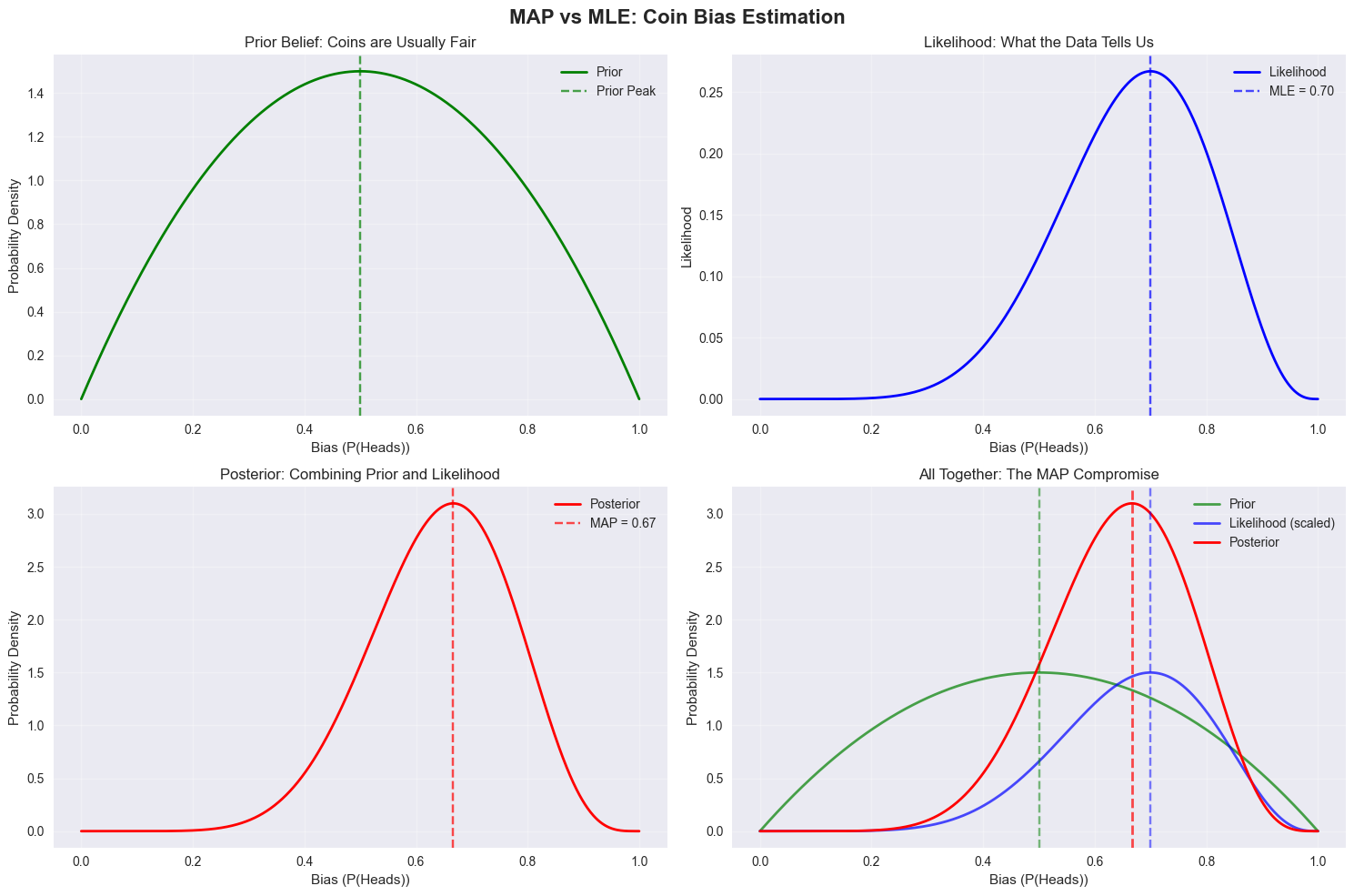
The amount of movement toward the prior depends on prior strength relative to the amount of data:

• With little data, a meaningful prior can substantially influence MAP.
• With abundant representative data, the likelihood dominates.
• With a uniform prior, MAP and MLE coincide.

This last fact follows immediately: if $p(\theta )$ is constant over the feasible parameter range, multiplying likelihood by that constant does not change its maximizer.

---

MAP as regularization

The connection between MAP and regularization is a frequent ML interview topic.

Assume a linear model with Gaussian noise:

$$y_i=w^{\top }{x}_i+{\epsilon }_i,{\epsilon }_i\sim \mathcal{N}(0,{\sigma }^2)$$

The negative log-likelihood is, up to constants:

$$\frac{1}{2{\sigma }^2}\sum _{i=1}^N(y_i-w^{\top }{x}_i{)}^2$$

Now place an independent zero-mean Gaussian prior on the weights:

$$w\sim \mathcal{N}(0,{\tau }^{2}I)$$

The negative log-prior is, up to constants:

$$\frac{1}{2{\tau }^2}\Vert w{\Vert }_2^2$$

The MAP objective is therefore:

$$\underset{w}{\min }\left[\frac{1}{2{\sigma }^2}\sum _{i=1}^N(y_i-w^{\top }{x}_i{)}^2+\frac{1}{2{\tau }^2}\Vert w{\Vert }_2^2\right]$$

This is ridge regression. A Gaussian prior centered at zero corresponds to an $L_2$ penalty that discourages large weights.

Similarly, independent Laplace priors lead to an $L_1$ penalty, which is the MAP interpretation behind lasso-style sparsity.

The concise interview statement is:

Regularization can be interpreted as a log-prior. Standard MLE minimizes negative log-likelihood, while MAP minimizes negative log-likelihood plus a penalty induced by prior beliefs about parameters.

Be precise about what this does not imply:

• A regularizer is only a Bayesian prior if it corresponds to a proper probabilistic prior under the stated model.
• A MAP estimate is one point estimate, not the complete posterior distribution.
• MAP is not necessarily the posterior mean. For skewed or multimodal posteriors, mean and mode can differ materially.

---

Choosing between MLE and MAP in practice

Question	MLE	MAP
Objective	Maximize $p(\mathcal{D}\mid \theta )$	Maximize $p(\theta \mid \mathcal{D})$
Uses a prior?	No	Yes
Optimization form	Maximize log-likelihood	Maximize log-likelihood plus log-prior
Small-data behavior	Can fit noise or produce extreme estimates	Can stabilize estimates if the prior is justified
Large-data behavior	Data dominates	Usually converges toward MLE with a fixed, well-behaved prior
Common ML connection	Cross-entropy and squared-error training	Regularization, smoothing, weight decay

For production ML, priors must be defensible. A prior could come from physics, known sensor behavior, historical versions of a system, or carefully separated historical datasets. It should not be a convenient way to force a preferred result.

For example, a prior based on the aggregate performance of an existing perception model might stabilize estimates for a rare night-rain-pedestrian slice. But if the new model architecture or data collection process changed substantially, that historical prior may no longer be appropriate. The system-level issue is not only mathematical: it is also a data lineage and distribution-shift question.

---

An interview-ready explanation

A compact but rigorous response could sound like this:

“MLE chooses parameters that maximize the likelihood of the observed data. Under independent samples, I maximize the sum of per-example log-likelihoods, or equivalently minimize negative log-likelihood. For a Bernoulli model, that gives the observed positive fraction; for a Gaussian model with fixed variance, it gives the sample mean.

MAP instead maximizes the posterior over parameters. By Bayes’ rule, that is likelihood times prior, so in log space it is the MLE objective plus a log-prior term. A Gaussian prior on weights produces $L_2$ regularization, so ridge regression has a MAP interpretation. MAP is especially useful when data are limited and the prior is justified; with a uniform prior, it reduces to MLE.”

---

Key takeaways

MLE estimates parameters using data alone:

$${\hat{\theta }}_{\mathrm{MLE}}=\arg \underset{\theta }{\max }p(\mathcal{D}\mid \theta )$$

For i.i.d. observations, maximize the log-likelihood instead:

$$\log p(\mathcal{D}\mid \theta )=\sum _{i=1}^N\log p(y_i\mid \theta )$$

For a Bernoulli model, MLE is the observed success rate:

$${\hat{\varphi }}_{\mathrm{MLE}}=\frac{H}{N}$$

MAP incorporates a prior:

$${\hat{\theta }}_{\mathrm{MAP}}=\arg \underset{\theta }{\max }\left[\log p(\mathcal{D}\mid \theta )+\log p(\theta )\right]$$

Conceptually, MAP is MLE with an explicit, probabilistically grounded regularization term. It can improve small-data estimates, but only when its prior assumptions are appropriate.

Next, you will move from parameter estimates to uncertainty around estimates by constructing and interpreting confidence intervals for model or experiment metrics.