Exact Diagonalization for Quantum Many-Body Systems

Recommended resources

The freely available resources this lesson will direct you to.

Hello! Welcome to the next lesson in our module on numerical methods for quantum systems.

In our previous lessons, we built powerful tools for simulating single-particle quantum mechanics. You learned to find stationary states by turning the time-independent Schrödinger equation into a matrix eigenvalue problem, and you simulated wavepacket dynamics using the Crank-Nicolson method for the time-dependent equation.

Now, we make the crucial leap from single-particle systems to the rich and complex world of many-body quantum mechanics. This is central to your goal of understanding condensed matter physics. Our first tool for tackling these systems is Exact Diagonalization (ED).

Your learning outcome for this lesson is to:

Apply exact diagonalization to calculate the ground state and low-lying excitations of a small quantum many-body system (e.g., a spin chain).

This method is the most direct way to solve a many-body problem. While it's limited to small systems, it is a foundational technique in computational physics, providing exact benchmarks against which more advanced approximate methods are tested.

1. From One Body to Many: The Challenge of Scale

The core idea of Exact Diagonalization is simple and familiar: we represent the Hamiltonian operator $H^$ as a matrix in a chosen basis and then numerically diagonalize it to find its eigenvalues (energies) and eigenvectors (the system's quantum states). This is precisely what you did for the single-particle Schrödinger equation.

The challenge with many-body systems is the size of the Hilbert space. For a single spin-1/2 particle, the space has dimension 2. For $N$ spin-1/2 particles, the states are tensor products, and the Hilbert space dimension grows as $2^{N}$ . This is known as the "curse of dimensionality".

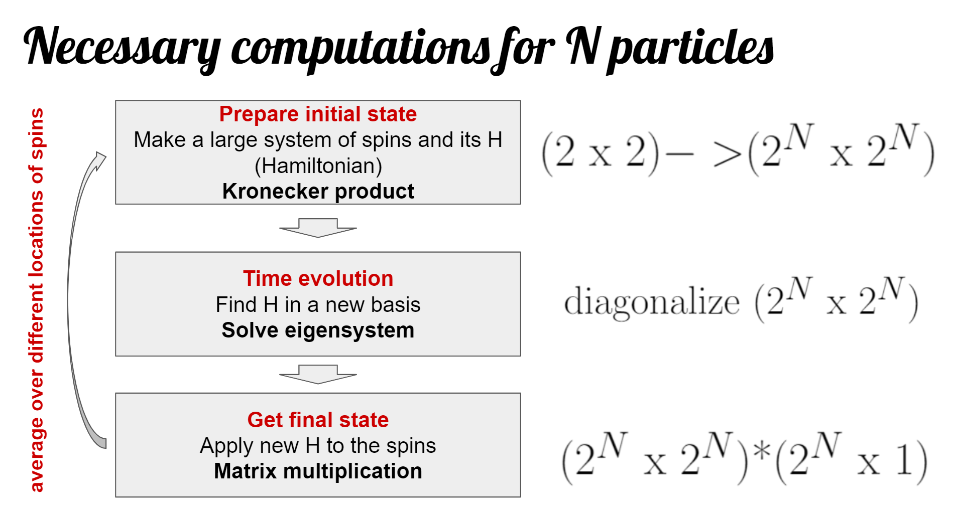
Computational Flow for N-Particle Spin Systems — This flowchart illustrates how the dimensions of the matrices involved in simulating a spin system grow exponentially with the number of particles, N. This exponential scaling is the fundamental limitation of exact diagonalization.

A system with just 30 spins has a Hilbert space of dimension $2^{30} \approx 1 0^{9}$ . Storing the corresponding Hamiltonian matrix would require thousands of terabytes of memory! ED is a "brute-force" method, and this exponential growth is why it's restricted to "small" systems (typically up to ~20-30 spins, and even fewer for more complex models).

Let's begin with a conceptual overview of what Exact Diagonalization entails.

Exact Diagonalization for spin systems

This video, 'Exact Diagonalization for spin systems' from Dr Mitchell's physics channel, provides an excellent introduction. It explains the core concept, its relation to solving the Schrödinger equation, and its primary limitation.

Please watch the introduction (00:00 - 04:26) and the final summary (55:19 - 58:13). Focus on the connection between solving the Schrödinger equation and diagonalizing the Hamiltonian matrix, and the role of the 'curse of dimensionality'.

2. The Algorithm: A Step-by-Step Guide for a Spin Chain

Let's make this concrete by developing the algorithm for the 1D Heisenberg model, a cornerstone model in magnetism. The Hamiltonian for nearest-neighbor interactions is:
$H^= J \sum_{i = 0}^{L - 2} S_{i} \cdot S_{i + 1} = J \sum_{i = 0}^{L - 2} (S_{i}^{z} S_{i + 1}^{z} + \frac{1}{2} (S_{i}^{+} S_{i + 1}^{-} + S_{i}^{-} S_{i + 1}^{+}))$
Here $L$ is the number of sites (spins). We will use the convention where $J > 0$ corresponds to an antiferromagnetic interaction (favoring anti-aligned spins) and $J < 0$ is ferromagnetic (favoring aligned spins).

The ED algorithm involves four main steps, which we'll implement for this Hamiltonian.

Exact Diagonalization for the 1D Heisenberg Chain

The article 'Exact Diagonalization for the 1D Heisenberg Chain' by Ryan Levy provides a clear, practical roadmap. We will follow its structure to build our understanding.

Read the 'Overview' section. It outlines the four key steps we will explore: (1) Generate the basis, (2) Generate the Hamiltonian Matrix, (3) Solve, and (4) Analyze.

Step 1: Representing the Basis

For a system of $L$ spin-1/2 particles, a natural basis is the set of all possible product states in the $S^{z}$ basis. For example, for $L = 3$ , one such state is $∣ ↑↓↑ ⟩$ .

For computational purposes, it's highly efficient to map these spin configurations to integers using a binary representation. A common convention is $∣ ↑ ⟩ \to 1$ and $∣ ↓ ⟩ \to 0$ .
$∣ ↑↓↑ ⟩ \to binary 101 \to integer 5$
This allows us to represent any basis state uniquely with an integer.

Step 2: Exploiting Symmetries (Block Diagonalization)

Constructing the full $2^{L} \times 2^{L}$ matrix is inefficient. We can do better. Notice that the Heisenberg Hamiltonian commutes with the total spin projection operator, $S^_{total}^{z} = \sum_{i} S^_{i}^{z}$ .
$[H^, S^_{total}^{z}] = 0$
This is a crucial observation. It means that the Hamiltonian does not connect states with different values of $S_{total}^{z}$ . Consequently, if we order our basis states according to their $S_{total}^{z}$ value, the Hamiltonian matrix becomes block diagonal. Each block corresponds to a subspace with a fixed number of up-spins (and thus a fixed $S_{total}^{z}$ ).

We can diagonalize each of these smaller blocks independently, which is computationally far cheaper.

Exact Diagonalization for spin systems

Let's return to Dr. Mitchell's video to see a formal explanation of how conserved quantum numbers lead to this block-diagonal structure.

Watch the segment on quantum numbers and block diagonalization (32:41 - 45:20). The key takeaway is that we can break the large diagonalization problem into several smaller, independent problems.

The process of generating a basis within a specific $S^{z}$ sector is the first practical step of an ED code.

Exact Diagonalization for the 1D Heisenberg Chain

This section of Ryan Levy's article shows how to implement this basis generation.

Read '1. Generate the basis'. Pay attention to the binary convention and the makeSzBasis function, which iterates through all possible integer states and groups them into lists based on their total S_z (which is determined by the number of set bits).

Step 3: Constructing the Hamiltonian Matrix

Now, for a specific $S_{total}^{z}$ block of size $D \times D$ , we need to compute the matrix elements $H_{mn} = ⟨ m ∣ H^∣ n ⟩$ , where $∣ m ⟩$ and $∣ n ⟩$ are basis states within that block.

Let's analyze the terms of $H^$ :

Diagonal Part ( $S_{i}^{z} S_{i + 1}^{z}$ ): The $S^{z}$ operator doesn't change a spin state, it only multiplies it by $\pm 1/2$ . So, when we apply this term to a basis state $∣ n ⟩$ , we get back the same state $∣ n ⟩$ multiplied by a number. This term only contributes to the diagonal elements $H_{nn}$ .
Off-Diagonal Part ( $S_{i}^{+} S_{i + 1}^{-} + S_{i}^{-} S_{i + 1}^{+}$ ): The raising and lowering operators flip spins. The term $S_{i}^{+} S_{i + 1}^{-}$ acts on a $∣ \dots ↓_{i} ↑_{i + 1} \dots ⟩$ configuration and turns it into $∣ \dots ↑_{i} ↓_{i + 1} \dots ⟩$ . This connects state $∣ n ⟩$ to a different state $∣ m ⟩$ , generating an off-diagonal element $H_{mn}$ . Notice that this operation conserves the total number of up spins, so $∣ m ⟩$ is in the same $S^{z}$ block as $∣ n ⟩$ .

Let's see this in action for the simplest non-trivial example: two spins.

Exact Diagonalization for spin systems

The video provides a crystal-clear, self-contained walkthrough for a two-spin system, showing exactly how the matrix blocks are constructed and diagonalized.

Watch the concrete example for two spins (45:20 - 55:19). Follow how the full 4x4 matrix is first constructed and then seen to be block-diagonal. Pay close attention to the diagonalization of the 2x2 block for the S_z=0 sector.

Step 4: Diagonalization and Analysis

Once a Hamiltonian block is constructed as a matrix (e.g., a numpy array), the final step is to find its eigenvalues and eigenvectors. Standard numerical libraries have highly optimized routines for this. In Python, numpy.linalg.eigh is ideal because it is designed for Hermitian matrices like our Hamiltonian.

The eigenvalues are the energies of the system's eigenstates within that $S^{z}$ sector. The eigenvectors represent those eigenstates, expressed as a superposition of our chosen basis states.

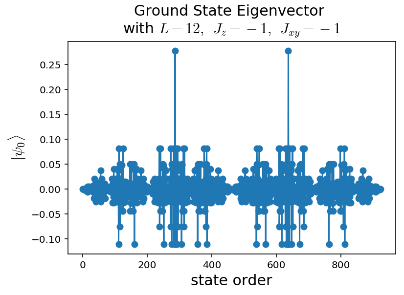
By collecting the eigenvalues from all $S^{z}$ blocks, we obtain the full energy spectrum. The lowest eigenvalue among all of them is the ground state energy. The corresponding eigenvector is the ground state wavefunction.

Ground State Eigenvector of a 1D Heisenberg Model — Components of the ground state eigenvector for an L=12 antiferromagnetic Heisenberg chain. The x-axis enumerates the basis states in the S_z=0 sector. Notice the ground state is a complex superposition of many different basis states, with the largest amplitudes corresponding to the classical antiferromagnetic (Neel) states and states with similar spin correlations.

3. Implementation and Advanced Concepts

You now have a complete conceptual picture of the ED algorithm. The provided article by Ryan Levy translates this directly into Python code.

Exact Diagonalization for the 1D Heisenberg Chain

Let's examine how the matrix construction and diagonalization are coded.

Read sections '2. Generate the Hamiltonian' and '3. Solve for the eigenvalues and eigenvectors'. In the makeH function, identify: The basisMap which maps a state's integer representation to its index in the matrix. The loop that calculates diagonal elements from S_z S_z terms. The else block that calculates off-diagonal elements from the spin-flipping terms. In the getSpectrum function, note the call to np.linalg.eigh(H), which performs the diagonalization.

For the system sizes we are considering, constructing and storing the entire Hamiltonian matrix block is feasible. For larger systems, this becomes impossible. More advanced ED codes use two key ideas:

Matrix Virtualization: The matrix elements are never stored. They are calculated "on-the-fly" as needed. This trades memory for computation.
Iterative Eigensolvers: Instead of diagonalizing the full matrix, algorithms like Lanczos can find the few lowest-lying (or highest-lying) eigenvalues and eigenvectors. This is done by repeatedly applying the Hamiltonian matrix to a random vector, which is very efficient when the matrix is sparse (has few non-zero elements), as the Heisenberg Hamiltonian is.

Given your background, it's good to be aware of these techniques, as they are essential for pushing ED to its limits.

On numerical methods in quantum spin systems - IDEALS

This chapter from a PhD thesis by A. G. Koch-Janusz, 'On numerical methods in quantum spin systems', provides a concise, high-level overview of the components and considerations for a professional ED implementation.

Skim through these sections to get a sense of the broader context. You don't need to absorb all the details, but focus on the concepts: Section 3.1: A summary of ED's pros (unbiased, exact) and cons (exponential scaling). Section 3.1.1: Reinforces the idea of basis representation and symmetry reduction. Section 3.1.2: Introduces matrix virtualization ('on-the-fly' evaluation). Section 3.1.3: Describes the Lanczos algorithm as a more efficient eigensolver for finding a few states.

Test your understanding!

Let's apply these concepts to a small but non-trivial system: a 4-site Heisenberg chain with open boundary conditions. Your task is to find the ground state in the $S_{total}^{z} = 0$ sector.

Instructions:

Generate the Basis:
- List all basis states for $L = 4$ that have $S_{total}^{z} = 0$ . (This means they must have two $∣ ↑ ⟩$ and two $∣ ↓ ⟩$ spins).
- How many such states are there? This will be the dimension of your Hamiltonian matrix.
- Represent each state as an integer (e.g., $∣ ↓↓↑↑ ⟩ \to 001 1_{2} = 3$ ).
Construct the Hamiltonian Matrix:
- Create a $D \times D$ matrix of zeros, where $D$ is the number of states you found in part 1.
- For simplicity, let $J = 1$ (the antiferromagnetic case).
- Calculate Diagonal Elements: For each state $∣ n ⟩$ , calculate $⟨ n ∣ H^∣ n ⟩$ . Remember, only the $S_{i}^{z} S_{i + 1}^{z}$ terms contribute. For each neighboring pair, parallel spins ( $↑↑, ↓↓$ ) contribute $+ 1/4$ , and anti-parallel spins ( $↑↓, ↓↑$ ) contribute $- 1/4$ . Sum these contributions over all three bonds ( $i = 0, 1, 2$ ).
- Calculate Off-Diagonal Elements: For each state $∣ n ⟩$ , apply the spin-flip terms $\frac{1}{2} \sum_{i} (S_{i}^{+} S_{i + 1}^{-} + S_{i}^{-} S_{i + 1}^{+})$ . If this connects $∣ n ⟩$ to another state in your basis, $∣ m ⟩$ , the matrix element $H_{mn}$ (and $H_{nm}$ ) will be $1/2$ .
Find the Ground State:
- You can use Python/Numpy (or your preferred tool) to diagonalize the resulting matrix.
- What is the ground state energy (the lowest eigenvalue)?
- What is the ground state eigenvector? Which basis states have the largest components in the ground state superposition? Does this make physical sense for an antiferromagnet?

Show answer

Basis States ( $S_{total}^{z} = 0$ ): There are $(2 4) = 6$ states. Let's order them by their integer representation:
- $∣ ↓↓↑↑ ⟩ \to 001 1_{2} = 3$ (index 0)
- $∣ ↓↑↓↑ ⟩ \to 010 1_{2} = 5$ (index 1)
- $∣ ↓↑↑↓ ⟩ \to 011 0_{2} = 6$ (index 2)
- $∣ ↑↓↓↑ ⟩ \to 100 1_{2} = 9$ (index 3)
- $∣ ↑↓↑↓ ⟩ \to 101 0_{2} = 10$ (index 4)
- $∣ ↑↑↓↓ ⟩ \to 110 0_{2} = 12$ (index 5)
Hamiltonian Matrix ( $J = 1$ ):
The resulting matrix should be:
$0.5 & 0.5 & 0 & 0 & 0 & 0 \\ 0.5 & -0.5 & 0.5 & 0.5 & 0 & 0 \\ 0 & 0.5 & 0.5 & 0 & 0.5 & 0 \\ 0 & 0.5 & 0 & 0.5 & 0.5 & 0 \\ 0 & 0 & 0.5 & 0.5 & -0.5 & 0.5 \\ 0 & 0 & 0 & 0 & 0.5 & 0.5 \end{pmatrix} $$$
Ground State:
- Diagonalizing this matrix yields the lowest eigenvalue (ground state energy) $E_{0} \approx - 1.2808$ .
- The corresponding eigenvector is approximately:
  $∣ ψ_{0} ⟩ \approx 0.23∣ ↓↓↑↑ ⟩ - 0.54∣ ↓↑↓↑ ⟩ + 0.36∣ ↓↑↑↓ ⟩ + 0.36∣ ↑↓↓↑ ⟩ - 0.54∣ ↑↓↑↓ ⟩ + 0.23∣ ↑↑↓↓ ⟩$
- The largest components correspond to states like $∣ ↓↑↓↑ ⟩$ and $∣ ↑↓↑↓ ⟩$ , which have the most "alternating" spin structure. This is physically intuitive for an antiferromagnet which favors anti-aligned nearest neighbors.

Conclusion

Congratulations! You have now worked through the entire process of solving a quantum many-body problem using Exact Diagonalization. This technique provides complete, unbiased information about the energy spectrum and eigenstates, making it an invaluable tool for small systems.

Key Takeaways:

Exact Diagonalization (ED) solves the many-body Schrödinger equation by representing the Hamiltonian as a matrix and numerically diagonalizing it.
The primary limitation is the curse of dimensionality, as the Hilbert space size $D$ grows exponentially with system size $N$ (e.g., $D = 2^{N}$ for spins).
Symmetries are crucial. Conserved quantities like $S_{total}^{z}$ allow the Hamiltonian to be block diagonalized, breaking one large problem into many smaller, manageable ones.
The ED algorithm consists of: (1) generating a basis for a symmetry sector, (2) constructing the Hamiltonian matrix elements for that block, and (3) using a numerical eigensolver to find energies and eigenstates.

Preview of the Next Lesson:

ED gives us the exact answer, but only for systems that are too small to exhibit many fascinating condensed matter phenomena like phase transitions. What happens when our system is too large for ED? We must turn to approximate methods. In the next lesson, you will learn about Variational Monte Carlo (VMC), a powerful method that uses statistical sampling to estimate the ground state properties of much larger systems.