Calculating Business Metrics in Excel

Hello. In the previous lesson, you learned how relative, absolute, and mixed references determine what happens when you copy a formula. That skill now becomes practical: a business analyst uses formulas to turn transaction-level data into metrics such as revenue, cost, profit, totals, and average performance.

In this lesson, you will build those metrics with Excel arithmetic and its core aggregate functions. The focus is not merely getting a number in a cell; it is making calculations dynamic, auditable, and meaningful for a business question.

---

From raw values to business metrics

A spreadsheet often begins with individual records: orders, invoices, expenses, products, employees, or customer interactions. A business metric summarizes or derives something useful from those records.

For example, an order dataset might contain:

Column	Meaning	Example
Order ID	Identifier for the order	ORD-1042
Unit Price	Price charged per item	25
Units	Quantity sold	12
Unit Cost	Cost per item	15

These values alone do not yet answer key questions. Formulas create the metrics:

Metric	Business meaning	Excel formula for row 4
Revenue	Money earned from the order	=B4*C4
Total Cost	Cost of all units in the order	=C4*D4
Gross Profit	Revenue remaining after direct costs	=E4-F4
Tax	Tax applied to profit, using a shared rate	=G4*$K$2
Net Profit	Profit after tax	=G4-H4

If row 4 has a unit price of 25, 12 units, and a unit cost of 15:

• Revenue is 25 * 12, or 300.
• Total cost is 12 * 15, or 180.
• Gross profit is 300 - 180, or 120.
• With an 8% tax rate in K2, tax is 120 * 8%, or 9.60.
• Net profit is 120 - 9.60, or 110.40.

The references in these formulas matter:

• B4, C4, and D4 are relative references, so they adjust for each new order row.
• $K$2 is an absolute reference, so every calculation uses the one approved tax-rate cell.

Avoid typing actual values directly into formulas, such as =25*12. That formula will not update if the source data changes. =B4*C4 remains connected to the spreadsheet’s data.

---

Arithmetic operators: the building blocks of row-level calculations

Every Excel formula begins with an equals sign, followed by cell references, numbers, operators, or functions.

The arithmetic operators you will use constantly are:

Purpose	Operator	Example	Typical analytical use
Addition	+	=E4+F4	Combine separate costs
Subtraction	-	=E4-F4	Calculate profit or variance
Multiplication	*	=B4*C4	Calculate revenue
Division	/	=E4/C4	Calculate revenue per unit
Percentage	%	=G4*8%	Apply a rate
Exponentiation	^	=2^3	Less common in basic business reporting

A few habits prevent many spreadsheet errors:

• Use * for multiplication, not the letter x.
• Use / for division.
• Store reusable assumptions, such as tax rates, commission rates, and targets, in clearly labelled cells.
• Format monetary outputs as Currency or Accounting, and rate inputs as Percentage. Formatting improves readability but does not change the underlying calculation.

If K2 contains 8%, Excel stores it as the decimal value 0.08. Therefore, =G4*$K$2 applies 8% correctly. Do not divide by 100 again.

Calculation order matters

Excel follows the normal order of operations:

1. Parentheses
2. Exponents
3. Multiplication and division
4. Addition and subtraction

This matters whenever one formula combines several operations.

Suppose revenue in E4 is 300, total cost in F4 is 180, and tax rate in K2 is 8%. To calculate tax on gross profit, the intended formula is:

=(E4-F4)*$K$2

Excel first calculates gross profit, 120, then applies 8% tax, producing 9.60.

Without parentheses:

=E4-F4*$K$2

Excel calculates F4*$K$2 first because multiplication has priority. It would subtract 14.40 from revenue, giving 285.60. That is not a tax calculation and is not a useful profit metric.

Use parentheses whenever the business meaning is “calculate this intermediate result first.”

---

Aggregate functions: summarize many records at once

Arithmetic formulas usually calculate one record at a time. For example, =B4*C4 calculates the revenue for one order.

An aggregate function summarizes a range of records. Its basic pattern is:

=FUNCTION(range)

For example:

=SUM(E4:E100)

This means: “Add every value from cell E4 through cell E100.”

The colon in E4:E100 means a continuous range. It is much clearer and safer than writing:

=E4+E5+E6+E7+...

The core aggregate functions are:

Function	What it returns	Example business question
SUM	Total of numeric values	What was total revenue?
AVERAGE	Arithmetic mean of numeric values	What was average revenue per order?
COUNT	Number of cells containing numbers	How many numeric sales entries were recorded?
COUNTA	Number of nonblank cells	How many order IDs are present?
MAX	Largest numeric value	What was the highest-value order?
MIN	Smallest numeric value	What was the lowest-value order?

For the example order sheet, a summary area might contain:

Summary metric	Formula
Total Revenue	=SUM(E4:E100)
Total Cost	=SUM(F4:F100)
Total Gross Profit	=SUM(G4:G100)
Total Net Profit	=SUM(I4:I100)
Average Revenue per Order	=AVERAGE(E4:E100)
Largest Order Revenue	=MAX(E4:E100)
Smallest Order Revenue	=MIN(E4:E100)
Number of Numeric Revenue Entries	=COUNT(E4:E100)
Number of Orders with an ID	=COUNTA(A4:A100)

The question should determine the function:

• “How much?” usually calls for SUM.
• “What is typical?” may call for AVERAGE.
• “How many numerical values are present?” calls for COUNT.
• “How many records have something entered?” can call for COUNTA.
• “What is the biggest or smallest value?” calls for MAX or MIN.

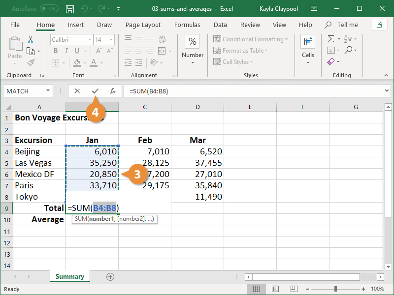
The displayed SUM example illustrates an important reporting pattern: retain detailed records in one area, then place metrics in a separate summary row or summary section. Do not include the summary cell itself in the range. A formula such as =SUM(E4:E101) placed in E101 creates a circular reference because Excel is being asked to include the result in its own calculation.

---

COUNT, COUNTA, blanks, and business interpretation

COUNT and COUNTA look similar, but they answer different questions.

Consider this order-ID column:

Cell	Value
A4	ORD-1001
A5	ORD-1002
A6	blank
A7	ORD-1004

• =COUNT(A4:A7) returns 0 because the order IDs are text, not numbers.
• =COUNTA(A4:A7) returns 3 because three cells are not blank.

Now consider Units Sold in C4:C7:

Cell	Value
C4	12
C5	8
C6	blank
C7	5

• =COUNT(C4:C7) returns 3.
• =SUM(C4:C7) returns 25.
• =AVERAGE(C4:C7) returns approximately 8.33 because Excel averages the three numeric values, not four rows.

That final behavior deserves attention. A blank might mean “data not entered,” “not applicable,” or “zero.” Those meanings are not interchangeable:

• If an order genuinely had zero units, enter 0.
• If the value is unknown or missing, do not casually replace it with zero.
• If a required metric is blank, flag it before relying on totals or averages.

You will learn systematic missing-value and error treatment in the next module. For now, recognize that aggregation functions are only as trustworthy as the values and ranges supplied to them.

MIN also needs interpretation. A minimum revenue of 0 may represent a legitimate zero-value order, a refund, a test record, or missing data that was incorrectly entered as zero. The formula finds the smallest value; the analyst determines what that value means.

---

Build a compact order-performance summary

A useful job-ready workflow is to calculate row-level metrics first, then summarize them.

Assume this worksheet layout:

Column	Header
A	Order ID
B	Unit Price
C	Units
D	Unit Cost
E	Revenue
F	Total Cost
G	Gross Profit
H	Tax
I	Net Profit

Put the tax-rate assumption in K2, label it clearly, and format it as Percentage.

For the first data row, enter these formulas:

Cell	Formula	Purpose
E4	=B4*C4	Revenue
F4	=C4*D4	Total direct cost
G4	=E4-F4	Gross profit
H4	=G4*$K$2	Tax using a fixed rate
I4	=G4-H4	Net profit

Fill the formulas down all transaction rows. Because the input references are relative, each row uses its own price, units, and cost. Because the tax-rate reference is absolute, every row uses the same tax assumption.

Below the data, create a small summary:

Cell label	Formula
Total Revenue	=SUM(E4:E100)
Total Gross Profit	=SUM(G4:G100)
Total Net Profit	=SUM(I4:I100)
Average Revenue per Order	=AVERAGE(E4:E100)
Highest Revenue Order	=MAX(E4:E100)
Orders Recorded	=COUNTA(A4:A100)

This layout supports a short performance update such as:

The dataset contains 97 recorded orders. Total revenue was 42,500, net profit was 8,100, and the average order generated approximately 438 in revenue. The highest-value order was 2,400.

The numbers are evidence. The interpretation must remain proportionate to what the data shows. For example, a high-value order is notable, but it does not by itself prove that a specific product, salesperson, or marketing activity caused the result.

---

A fast formula-quality check

Before sharing calculations, use this short review routine:

1. Read the formula, not just the displayed value. Select a calculated cell and inspect the Formula Bar.
2. Inspect a copied cell away from the first row. Confirm that row-level references changed as expected and shared assumptions remained fixed.
3. Check the selected range. A total should cover data rows, not headings, other summaries, or unrelated values.
4. Compare a total with a visible subset. Select a few values and use Excel’s status bar as a quick reasonableness check.
5. Use sensible formatting. Currency for money, Percentage for rates, and an appropriate number of decimal places make metrics readable.
6. Look for suspicious values. Zeros, blanks, very large results, negative profit, and #DIV/0! errors should be investigated rather than ignored.

Formula auditing is part of analysis, not a final cosmetic step. A precisely calculated answer to the wrong range is still the wrong answer.

---

Key takeaways and next step

Excel arithmetic converts record-level inputs into operational metrics:

• Use +, -, *, and / to calculate values such as revenue, cost, profit, and per-unit measures.
• Use parentheses to make the intended business logic explicit when a formula has several operations.
• Use cell references instead of hard-coded values so calculations update with the data.
• Use SUM, AVERAGE, COUNT, COUNTA, MAX, and MIN to summarize a dataset.
• Distinguish a formula’s calculation from its interpretation: blanks, zeros, and unusually high or low values require business context.
• Keep detailed data and summary metrics separate, and validate ranges before reporting results.

Next, you will apply IF logic to categorize records according to a business rule, such as marking orders as “High Value,” “On Target,” or “Needs Review.”