The Ginzburg Criterion

Recommended resources

The freely available resources this lesson will direct you to.

Hello! Welcome to the next lesson in our journey through the statistical mechanics of phase transitions.

In our previous lessons, we have built up the Landau-Ginzburg theory, which describes a system in terms of a spatially varying order parameter field $m (r)$ . We've explored this theory from two different angles:

Mean-Field Theory: By finding the uniform field $m_{0}$ that minimizes the free energy (the saddle-point approximation), we recovered the classical mean-field critical exponents. This approach completely ignores fluctuations.
Fluctuation Effects: By considering small fluctuations around the mean-field state (the Gaussian approximation), we calculated the correlation function and found that the correlation length $ξ$ diverges at the critical point. We also saw how large, non-linear fluctuations can form stable domain walls.

These analyses lead to a crucial question: if fluctuations are so important near the critical point, when can we ever trust the simple mean-field theory we spent time developing? This lesson is dedicated to answering exactly that. We will derive the Ginzburg criterion, a powerful condition that tells us when mean-field theory provides a valid description of a system.

Our objective is to quantify the competition between the ordered state predicted by mean-field theory and the thermal fluctuations that tend to disrupt it. By comparing their relative magnitudes, we will discover the crucial role of spatial dimensionality and arrive at the concept of the upper critical dimension.

The Core Idea: Fluctuations vs. Mean Value

The Ginzburg criterion is based on a simple, physical idea. Mean-field theory is a good approximation if the system is, on average, close to the predicted mean-field state. Let's consider the system below the critical temperature, $T < T_{c}$ . Mean-field theory predicts a non-zero, uniform order parameter $m_{0}$ . However, thermal fluctuations mean that the actual local order parameter $m (r)$ will deviate from this value.

The criterion for the validity of mean-field theory is that these fluctuations must be small compared to the mean value itself. Mathematically, we require that the mean-squared fluctuation of the order parameter is much smaller than the square of the mean-field order parameter:

⟨ (m (r) - m_{0})^{2} ⟩ ≪ m_{0}^{2}

Or, letting $δ m (r) = m (r) - m_{0}$ , we need:

⟨(δ m)^{2} ⟩ ≪ m_{0}^{2}

Our task is to calculate the left-hand side of this inequality and see under what conditions the inequality holds, particularly as we approach the critical temperature $T_{c}$ .

Deriving the Ginzburg Criterion

The derivation involves estimating the magnitude of the thermal fluctuations, $⟨(δ m)^{2} ⟩$ , and comparing it to the mean-field value $m_{0}^{2}$ . The following video provides a very clear, step-by-step walkthrough of this derivation using a physical "patch" or "domain" argument that is quite intuitive.

Landau Ginzburg theory of Phase Transitions

Please watch this section from Jos Thijssen's lecture on Landau-Ginzburg theory. It provides a complete derivation of the Ginzburg criterion, starting from its conceptual basis and ending with the final condition involving the system's dimensionality.

Watch the video segment from 33:54 to 47:17. Focus on how the argument proceeds: Stating the criterion: fluctuations must be small compared to the mean value. Estimating the local fluctuation (\langle (\delta m_r)^2 angle) by relating it to the fluctuations of the total magnetization over a correlation volume \xi^d. Substituting the known mean-field dependencies for the correlation length \xi and the order parameter m_0 as a function of the reduced temperature t. Analyzing the final inequality to determine for which dimensions d the criterion holds near T_c.

Let's summarize the key steps and results from the video.

1. Estimating the Fluctuations

The central physical insight is that the system can be viewed as being composed of roughly independent patches of volume $V_{ξ} \sim ξ^{d}$ , where $ξ$ is the correlation length. The average fluctuation of the order parameter within one such patch gives an estimate of the typical local fluctuation $⟨(δ m)^{2} ⟩$ .

The fluctuation of the order parameter averaged over a volume $V$ is related to the susceptibility $χ$ through the fluctuation-dissipation theorem: $⟨(δ m_{V})^{2} ⟩ = \frac{k _{B} T χ}{V}$ .
Applying this to a correlation volume $V_{ξ}$ , we get our estimate for the local fluctuation:

⟨(δ m)^{2} ⟩ \approx \frac{k _{B} T χ}{ξ ^{d}}

2. Substituting Mean-Field Scaling

Now, we substitute the behavior of $m_{0}$ , $χ$ , and $ξ$ near the critical point, as predicted by mean-field theory. Let $t = \frac{T - T _{c}}{T _{c}}$ be the reduced temperature. For $T < T_{c}$ , we have $t < 0$ .

Order Parameter: $m_{0}^{2} = - \frac{a _{0}}{b _{0}} = - \frac{a t}{b _{0}} \propto ∣ t ∣$ . (This implies the critical exponent $β = 1/2$ ).
Correlation Length: $ξ^{2} = \frac{κ}{- 2 a _{0}} = \frac{κ}{- 2 a t} \propto ∣ t ∣^{- 1}$ . (This implies the exponent $ν = 1/2$ ).
Susceptibility: $χ = \frac{1}{- 2 a _{0}} = \frac{1}{- 2 a t} \propto ∣ t ∣^{- 1}$ . (This implies the exponent $γ = 1$ ).

3. Forming the Ratio

We can now substitute these scaling relations into our criterion $⟨(δ m)^{2} ⟩ ≪ m_{0}^{2}$ . Let's examine the ratio $R = \frac{⟨( δ m ) ^{2} ⟩}{m _{0}^{2}}$ :

R \propto \frac{χ / ξ ^{d}}{m _{0}^{2}} \propto \frac{∣ t ∣ ^{- 1} / ( ∣ t ∣ ^{- 1/2} ) ^{d}}{∣ t ∣ ^{1}} = \frac{∣ t ∣ ^{- 1}}{∣ t ∣ ^{- d /2} ∣ t ∣ ^{1}} = ∣ t ∣^{d /2 - 2} = ∣ t ∣^{(d - 4) /2}

The condition for mean-field theory to be valid is $R ≪ 1$ .

4. The Role of Dimensionality

The behavior of this ratio as we approach the critical point ( $t \to 0$ ) depends crucially on the sign of the exponent $(d - 4) /2$ :

If $d > 4$ : The exponent is positive. As $t \to 0$ , the ratio $R \to 0$ . This means that fluctuations become less important relative to the mean-field value as we get closer to the critical point. In this case, mean-field theory becomes exact at criticality and provides a correct description of the critical exponents.
If $d < 4$ : The exponent is negative. As $t \to 0$ , the ratio $R \to \infty$ . The fluctuations completely overwhelm the mean-field order parameter. Mean-field theory catastrophically fails near the critical point, and the critical exponents it predicts will be incorrect.
If $d = 4$ : The exponent is zero, and the ratio $R$ approaches a constant (with possible logarithmic corrections that we've ignored). Fluctuations are significant but do not overwhelm the system in the same way. This limiting dimension is called the upper critical dimension, $d_{c} = 4$ , for this universality class (e.g., Ising magnets, liquid-gas transitions).

The following resources provide excellent complementary discussions of this derivation and its implications.

[PDF] 2. My First Path Integral

For a concise and elegant restatement of the argument, please read the relevant section from David Tong's lecture notes. It approaches the derivation from a slightly different but equivalent angle, reinforcing the main result.

Read Section 2.2.4, 'The Upper Critical Dimension'. Notice how it estimates the ratio of the integrated fluctuation to the integrated mean value within a correlation volume, arriving at the same scaling relation R \propto |t|^{(d-4)/2}.

[PDF] Chapter 2 Ginzburg-Landau Phenomenology

To connect this theoretical result to experimental reality, this resource introduces the 'Ginzburg temperature' and discusses why mean-field theory works beautifully for some systems (like conventional superconductors) but not others.

Read Section 2.8, 'Ginzburg Criterion'. This section defines the reduced temperature t_G where fluctuations become important. Pay attention to the argument for why t_G is experimentally inaccessible for superconductors but accessible for superfluids like liquid helium, explaining why the former appear to follow mean-field theory perfectly.

Application: Ginzburg Criterion for a Polymer Blend

Your background includes work on soft matter systems, which often provide textbook examples of the concepts we're studying. Let's apply what we've learned to a new system: a symmetric polymer blend. The following problem walks you through the derivation of the Ginzburg criterion starting from the Flory-Huggins free energy, which is a cornerstone of polymer physics.

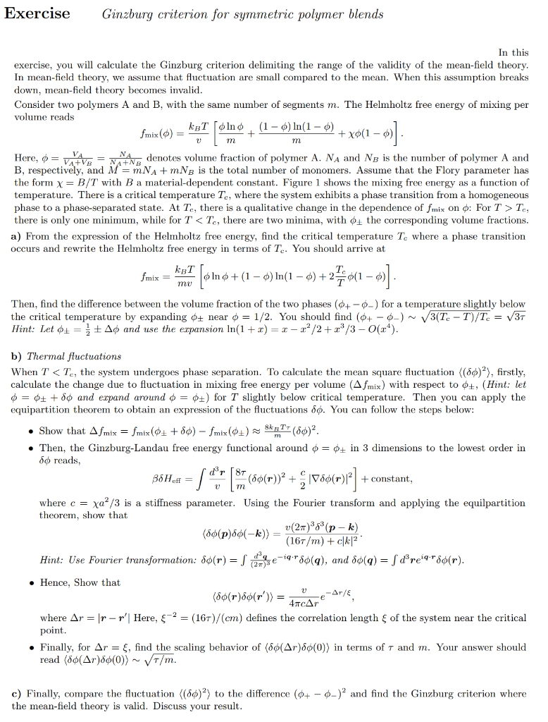
Exercise: Ginzburg Criterion for Symmetric Polymer Blends — CAPTION: An exercise detailing the steps to derive the Ginzburg criterion for a symmetric polymer blend. It involves finding the critical temperature, calculating the mean-square fluctuation from the Helmholtz free energy, and finally comparing the fluctuation magnitude with the mean-field prediction to establish the criterion. Source: Chegg Inc.

Take some time to work through this problem. It is an excellent way to solidify your understanding. You will see how the general Landau-Ginzburg framework and the Ginzburg criterion can be applied to a specific physical model by first performing a Taylor expansion of the system's specific free energy around the critical point to map it onto the general $ϕ^{4}$ form.

Hints for the exercise

Part (a): The critical point is found by setting the second and third derivatives of the free energy density with respect to the order parameter $ϕ$ to zero. $\frac{\partial ^{2} f}{\partial ϕ ^{2}} = 0$ and $\frac{\partial ^{3} f}{\partial ϕ ^{3}} = 0$ . This will give you the critical interaction parameter $χ_{c}$ and critical composition $ϕ_{c}$ .
Part (b): You need to expand the free energy functional around the critical point $ϕ_{c}$ . The result will look like a Landau-Ginzburg functional. The coefficient of the $(\nabla ϕ)^{2}$ term (the gradient term) is given in the problem as $κ$ .
Part (c): Use the result $⟨(δ ϕ)^{2} ⟩ \approx \frac{k _{B} T χ}{ξ ^{d}}$ . You will need to find the expressions for $χ$ and $ξ$ from the coefficients of your Landau-Ginzburg expansion from part (b). Remember that near $T_{c}$ , $χ \approx χ_{c} (1 - T / T_{c})$ .
Part (d): The mean-field order parameter $ϕ_{0}$ below $T_{c}$ is found by minimizing the expanded free energy. Its square will be proportional to $∣ T - T_{c} ∣$ .
Part (e): Form the ratio $\frac{⟨( δ ϕ ) ^{2} ⟩}{ϕ _{0}^{2}}$ and find the condition for it to be much less than 1. This will give you the Ginzburg criterion in terms of the molecular parameters $N$ and $a$ .

Conclusion

Key Takeaways:

The Ginzburg criterion provides a quantitative test for the validity of mean-field theory by comparing the magnitude of thermal fluctuations to the mean-field value of the order parameter.
Mean-field theory is valid when $⟨(δ m)^{2} ⟩ ≪ m_{0}^{2}$ .
This inequality leads to the condition $∣ t ∣^{(d - 4) /2} ≪ 1$ , where $t$ is the reduced temperature and $d$ is the spatial dimensionality.
The dimension $d_{c} = 4$ is the upper critical dimension for systems in the Ising universality class.
- Above $d_{c}$ , mean-field theory works and its exponents are correct.
- Below $d_{c}$ , fluctuations dominate near $T_{c}$ , and mean-field theory breaks down.
Even for $d < 4$ , mean-field theory can be a good approximation if the system is not too close to the critical point, i.e., for $∣ t ∣ > t_{G}$ , where $t_{G}$ is the Ginzburg temperature.

We have now established a fundamental limitation of our simplest theoretical model. This is not a failure, but a signpost pointing the way forward. The breakdown of mean-field theory in realistic dimensions ( $d = 2, 3$ ) tells us that a more sophisticated approach is needed to handle the dominant role of fluctuations at criticality.

Preview of the Next Lesson:

Having established that MFT is only valid above $d = 4$ , we need a way to find the correct critical exponents for $d < 4$ . We also need a framework to understand why systems as different as a magnet and a fluid can share the same exponents. The next two concepts we will explore, scaling and universality, provide the phenomenological answer to these questions. We will postulate so-called "scaling laws" that relate different critical exponents and introduce the idea of universality classes, setting the stage for the powerful machinery of the Renormalization Group.