Order Parameters, Correlation, and Criticality

Recommended resources

The freely available resources this lesson will direct you to.

[PDF] Phase transitions and critical phenomena - UBC Physics & Astronomyphas.ubc.ca
[PDF] Phase Transitions and Collective Phenomena - TCM Groupwww.tcm.phy.cam.ac.uk

Hello! Welcome to the next stage of our journey into the statistical mechanics of phase transitions.

In the previous module, we developed Landau's phenomenological theory, a powerful framework for describing phase transitions based on symmetry arguments and an expansion of the free energy in a spatially uniform order parameter. We saw how it could be applied to complex systems like crystals undergoing structural transitions.

However, a key simplification in Landau theory is the assumption that the order parameter is uniform in space. This is equivalent to neglecting spatial fluctuations, which, as we'll see, become the dominant feature of a system near its critical point. Before we move to specific microscopic models like the Ising model (which I mentioned in the last preview), it's more logical to first extend Landau's phenomenological approach to include these crucial spatial variations. This extension is known as Landau-Ginzburg theory, which we will begin exploring in this module.

Our first step is to develop the language needed to describe these fluctuations. Today's lesson focuses on this foundational task. The learning outcome is to: define the order parameter correlation function and correlation length, and explain their behavior at criticality. These two concepts are the cornerstones for understanding the physics of fluctuations and the emergence of universal behavior near a phase transition.

1. Fluctuations and the Correlation Function

In our previous discussions, we minimized a free energy F(m) to find a single, uniform equilibrium value for the order parameter, $\overset{m}{ˉ}$ . In reality, the local order parameter $m (r)$ is not constant; it fluctuates in space around this average value. Think of a magnet above its Curie temperature: on average, the magnetization is zero, but at any instant, there are fluctuating patches of local "spin-up" and "spin-down" regions.

The fundamental question is: how are the fluctuations at one point $r$ related to the fluctuations at another point $r^{'}$ ? The two-point correlation function provides the answer. For a translationally invariant system, we define the connected correlation function as:

G_{c} (r) = ⟨ δ m (r) δ m (0)⟩ \equiv ⟨(m (r) - \overset{m}{ˉ}) (m (0) - \overset{m}{ˉ})⟩ = ⟨ m (r) m (0)⟩ - \overset{m}{ˉ}^{2}

Here, $\overset{m}{ˉ} = ⟨ m (r)⟩$ is the average value of the order parameter, and $δ m (r) = m (r) - \overset{m}{ˉ}$ is the local fluctuation.

If $G_{c} (r) > 0$ , a fluctuation at the origin makes a fluctuation in the same direction at position $r$ more likely.
If $G_{c} (r) < 0$ , the fluctuations tend to be opposite (relevant for things like antiferromagnets).
If $G_{c} (r) = 0$ , the fluctuations are statistically independent.

The following reading provides a concrete derivation of the correlation function and connects it to the magnetic susceptibility, a relationship we will explore more deeply in the next lesson.

[PDF] Phase Transitions and Collective Phenomena - TCM Group

The section 'Long-range Correlations' in the notes from the TCM Group at Cambridge provides an excellent, self-contained introduction to the connected correlation function.

Please read the subsection '1.3.4 Long-range Correlations'. Focus on the definition of the 'connected' correlation function, Gc(x), and the physical intuition that it measures how local fluctuations affect each other. Note the final sentence which states its importance in defining the correlation length.

2. The Correlation Length, $ξ$

In a typical system away from a phase transition, the influence of a fluctuation at one point dies off quickly with distance. We expect the correlation function $G_{c} (r)$ to decay to zero for large $∣ r ∣$ . This decay is characterized by a fundamental length scale: the correlation length, $ξ$ .

For large distances ( $∣ r ∣ ≫ ξ$ ), the correlation function in many systems is well-described by an exponential decay:

G_{c} (r) \sim e^{- ∣ r ∣/ ξ}

The correlation length $ξ$ represents the typical spatial extent of a coherent fluctuation. You can think of it as the "range of influence" of a local fluctuation or the average size of correlated domains in the system.

3. Divergence of the Correlation Length at Criticality

The behavior of the correlation length is what makes critical phenomena so fascinating. As a system with a continuous phase transition approaches its critical temperature $T_{c}$ , the correlation length diverges.

ξ (T) \to \infty as T \to T_{c}

This divergence is described by a new critical exponent, $ν$ (nu):

ξ \propto ∣ t ∣^{- ν}

where $t = (T - T_{c}) / T_{c}$ is the reduced temperature. In mean-field theories, such as the one we will derive from the Landau-Ginzburg functional, we will find that $ν = 1/2$ .

Correlation Length Divergence at Criticality — Plots of the correlation length $\xi(t)$ for the binary fluid nitroethane-cyclohexane near its critical point. (a) A linear-log plot showing the sharp increase as the reduced temperature $t$ approaches zero. (b) A log-log plot revealing a straight line, which is the signature of the power-law divergence $\xi \propto |t|^{-\nu}$. The slope of this line gives $-\nu$. Image from a presentation by G. Ahlers, UCSB.

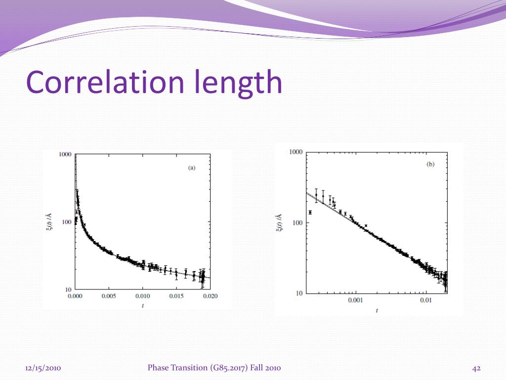
The divergence of $ξ$ is the central event at a critical point. It means that fluctuations become correlated over all length scales, from the microscopic lattice spacing up to the size of the entire system. This scale-invariance is the reason why microscopic details become irrelevant at criticality and systems as different as a liquid-gas fluid and a ferromagnet can exhibit the same critical exponents—the phenomenon of universality.

4. Correlation Function at the Critical Point

If $ξ \to \infty$ , what happens to the correlation function $G_{c} (r)$ precisely at $T = T_{c}$ ? An exponential decay $e^{- ∣ r ∣/\infty}$ is meaningless. Instead, the decay becomes much slower, changing from exponential to a power law:

G_{c} (r) \propto \frac{1}{∣ r ∣ ^{d - 2 + η}} (at T = T_{c})

Here, $d$ is the spatial dimensionality of the system, and we have introduced another new critical exponent, $η$ (eta), often called the "anomalous dimension."

Away from $T_{c}$ : Correlation is short-ranged ( $ξ$ is finite) and decays exponentially.
At $T_{c}$ : Correlation is long-ranged ( $ξ$ is infinite) and decays algebraically (as a power law).

In simple mean-field theories, $η = 0$ , so the decay is predicted to be $1/∣ r ∣^{d - 2}$ . The fact that experiments and more exact theories (like the 2D Ising model solution) find a small, non-zero $η$ is a key failure of mean-field theory, pointing to the importance of a more sophisticated treatment of fluctuations.

5. Correlations in Fourier Space: The Structure Factor

The correlation function is most directly probed in scattering experiments (e.g., neutron scattering for magnets, light scattering for fluids). These experiments don't measure $G_{c} (r)$ directly, but rather its Fourier transform, known as the static structure factor, $S (q)$ .

S (q) = \int d^{d} r e^{- i q \cdot r} G_{c} (r)

A common and highly useful approximation for the structure factor near a critical point is the Ornstein-Zernike (OZ) form:

S (q) \propto \frac{1}{q ^{2} + ξ ^{- 2}}

where $q = ∣ q ∣$ is the magnitude of the wavevector. Let's see how this simple expression beautifully captures the physics:

Away from $T_{c}$ ( $ξ$ is finite): $S (q)$ is a Lorentzian function of $q$ . The peak at $q = 0$ has a height proportional to $ξ^{2}$ , and its width is proportional to $1/ ξ$ . As $T \to T_{c}$ , the peak grows taller and narrower.
At $T_{c}$ ( $ξ \to \infty$ ): The $ξ^{- 2}$ term vanishes, and the structure factor takes a simple power-law form: $S (q) \propto \frac{1}{q ^{2}}$ This corresponds to the real-space power-law decay $G_{c} (r) \propto 1/∣ r ∣^{d - 2}$ (i.e., the mean-field case where $η = 0$ ). The more general form including $η$ is $S (q) \propto 1/ q^{2 - η}$ .

The following resources provide a more formal derivation of these results from the Landau-Ginzburg perspective, which we will tackle in upcoming lessons.

[PDF] Phase Transitions and Collective Phenomena - TCM Group

These two texts discuss the form of the correlation function in both real and Fourier space. The first, which you've already opened, shows the derivation within the Landau-Ginzburg framework, while the second provides a concise summary.

Please read section '2.6 Fluctuations, Correlations & Susceptibilities' (up to the end of page 28). Pay close attention to how the correlation lengths \xi_l, \xi_t are defined (Eq. 2.21), the Ornstein-Zernike form of the correlation function in Fourier space (Eq. 2.22), and its asymptotic real-space behavior (Eq. 2.24). Note the critical exponent ( u=1/2) that emerges.

[PDF] Phase transitions and critical phenomena - UBC Physics & Astronomy

This document from UBC Physics & Astronomy offers a very compact overview of the key results for the correlation function.

Read the introductory paragraph on page 3 and section '3.3 Correlations'. This will reinforce the definitions of \xi and ( u), the Ornstein-Zernike form ( ilde{G}(q)), and the asymptotic real-space behavior of G_c(r).

Test your understanding!

A light scattering experiment on a binary fluid mixture near its critical point measures the scattered intensity $I$ as a function of the scattering wavevector $q$ . At a given temperature $T$ , the data is well-described by the Lorentzian (Ornstein-Zernike) form:

I (q, T) = \frac{I _{0}}{q ^{2} + k ( T ) ^{2}}

As the temperature is varied towards the critical temperature $T_{c}$ , the parameter $k (T)$ is observed to vanish following a power law: $k (T) \propto ∣ T - T_{c} ∣^{0.63}$ .

How is the experimentally determined parameter $k (T)$ related to the theoretical concepts we discussed today?
What is the value of the critical exponent $ν$ for this system? Is it consistent with mean-field theory?

Show answer

Comparing the experimental form $I (q) \propto 1/ (q^{2} + k^{2})$ with the theoretical Ornstein-Zernike form for the structure factor $S (q) \propto 1/ (q^{2} + ξ^{- 2})$ , we can directly identify that the parameter $k (T)$ is the inverse of the correlation length: $k (T) = 1/ ξ (T)$ .
We are given that $k (T) \propto ∣ T - T_{c} ∣^{0.63}$ . Since $k = 1/ ξ$ , this implies $ξ (T) \propto (∣ T - T_{c} ∣^{0.63})^{- 1} = ∣ T - T_{c} ∣^{- 0.63}$ .
By comparing this with the definition $ξ \propto ∣ T - T_{c} ∣^{- ν}$ , we find that the critical exponent for this system is $ν = 0.63$ .
This value is not consistent with the mean-field prediction of $ν = 1/2 = 0.5$ . The measured value is characteristic of the 3D Ising universality class, which accurately describes the liquid-gas and binary fluid critical points.

Conclusion

Key Takeaways:

Near a phase transition, it is essential to consider spatial fluctuations of the order parameter, $m (r)$ .
The connected correlation function, $G_{c} (r) = ⟨ m (r) m (0)⟩ - \overset{m}{ˉ}^{2}$ , quantifies the statistical relationship between fluctuations at different points.
The correlation length, $ξ$ , is the characteristic distance over which these fluctuations are correlated. Away from criticality, $G_{c} (r)$ decays exponentially with a rate of $1/ ξ$ .
At a continuous phase transition, the correlation length diverges as a power law: $ξ \propto ∣ t ∣^{- ν}$ . This is the defining feature of criticality.
At the critical point itself, the correlation function decays much more slowly, as a power law: $G_{c} (r) \propto 1/∣ r ∣^{d - 2 + η}$ .
In Fourier space, these behaviors are captured by the Ornstein-Zernike form of the structure factor, $S (q) \propto 1/ (q^{2} + ξ^{- 2})$ , which is directly measurable in scattering experiments.

Preview of the Next Lesson:

We have now defined the essential language for describing fluctuations. In the next lesson, we will formalize the connection between fluctuations and thermodynamic response functions by deriving the fluctuation-dissipation theorem, which relates the susceptibility $χ$ to the integral of the correlation function $G_{c} (r)$ . This will make it clear why a diverging correlation length necessarily implies a diverging susceptibility.