From Band Dispersion to DOS: Van Hove Singularities

Hello! Welcome to our next lesson.

In our previous session, we established a powerful numerical framework for computing the band structure, $E_n(\mathbf{k})$, for any given tight-binding model. We saw how a complete map of the energy bands can be generated by diagonalizing the Bloch Hamiltonian along high-symmetry paths in the Brillouin zone.

Today, we'll build directly on that foundation. Knowing the energy of every possible electron state is useful, but many physical properties depend not on the energy of a specific state, but on how many states are available at a particular energy. This leads us to one of the most fundamental quantities in solid-state physics: the electronic density of states (DOS).

Our goal is to learn how to calculate the DOS from a given band dispersion, $E(\mathbf{k})$, and to identify special features within it known as van Hove singularities. The DOS is not just a theoretical construct; it is directly linked to measurable properties like optical absorption and tunneling conductance, making it a crucial bridge between theory and experiment.

1. Defining the Density of States

The density of states, $g(E)$, is defined as the number of available electronic states per unit energy, per unit volume (or area/length in lower dimensions).

Formally, if we have $N(E)$ total states with energy less than $E$, the DOS is its derivative:

where $V$ is the volume of the crystal.

To calculate this from a band structure $E(\mathbf{k})$, we need to count how many $\mathbf{k}$-states correspond to a given energy $E$. This counting can be expressed elegantly using the Dirac delta function. For a single band in $D$ dimensions, the DOS is:

where $g_s$ is a degeneracy factor (e.g., $g_s=2$ for spin), and the integral is over the first Brillouin zone (BZ). The delta function enforces the condition that we only "count" the $\mathbf{k}$ points that have the energy $E$.

A more intuitive, and often more useful, form of this equation can be derived by transforming the integral over the entire BZ into a surface integral over a surface of constant energy $S(E)$ in $\mathbf{k}$-space.

The central result from this reading is the expression for the density of states as an integral over the constant-energy surface $S(E)$:

This equation is profoundly important. It tells us that the contribution to the DOS from a region in $\mathbf{k}$-space is inversely proportional to the magnitude of the group velocity, $v_g=\frac{1}{\hslash }|{\nabla }_{\mathbf{k}}E(\mathbf{k})|$. Where the bands are flat (${\nabla }_{\mathbf{k}}E\to 0$), the group velocity is small, and these states contribute heavily to the density of states.

2. Van Hove Singularities

The surface integral formula immediately reveals that something dramatic must happen at points in the Brillouin zone where ${\nabla }_{\mathbf{k}}E(\mathbf{k})=0$. These are the critical points of the band structure:

• Local minima (e.g., the bottom of a band)
• Local maxima (e.g., the top of a band)
• Saddle points

At these critical points, the denominator in the integrand goes to zero, causing the DOS, or its derivative, to diverge. These special features are called van Hove singularities. Their shape depends on the dimensionality of the system.

To summarize the key points on the nature of these singularities:

• In 3D: The DOS has kinks where its derivative is discontinuous, typically showing a square-root dependence $g(E)\sim \sqrt{|E-E_c|}$ near a band edge $E_c$.
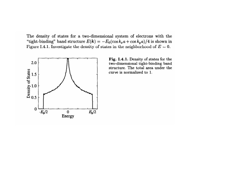
• In 2D: At a band minimum or maximum, the DOS has a step-function discontinuity. At a saddle point, it has a much stronger logarithmic divergence, $g(E)\sim \ln |E-E_c|$.
• In 1D: The DOS itself diverges at band edges as $g(E)\sim |E-E_c{|}^{-1/2}$.

The 2D logarithmic singularity is a classic example. Consider the simple tight-binding model on a square lattice, $E(k_x,k_y)=-2t(\cos (k_{x}a)+\cos (k_{y}a))$. This dispersion has a saddle point at $(\pi /a,0)$ and $(0,\pi /a)$ corresponding to $E=0$. This leads to a sharp, divergent peak in the DOS at the band center.

3. Calculating the DOS for Simple Dispersions

Let's now apply these concepts to derive the functional form of the DOS for simple, isotropic band structures of the form $E(\mathbf{k})=C|\mathbf{k}{|}^{\alpha }$, where $\alpha$ is a constant. This covers common cases like parabolic bands ($\alpha =2$) and linear bands ($\alpha =1$, like in graphene).

The following video provides a clear, general derivation for any dimension $D$ and any exponent $\alpha$.

The video's derivation leads to a powerful result: for a dispersion $E\propto k^{\alpha }$ in $D$ dimensions, the density of states behaves as:

Let's apply this to the case of a standard parabolic band ($\alpha =2$, e.g., free electrons or states near a band minimum):

• 3D (D=3): $g(E)\propto E^{\frac{3}{2}-1}=E^{1/2}$. This is the classic square-root dependence for bulk materials.
• 2D (D=2): $g(E)\propto E^{\frac{2}{2}-1}=E^0=\text{constant}$. The DOS for a 2D electron gas is constant.
• 1D (D=1): $g(E)\propto E^{\frac{1}{2}-1}=E^{-1/2}$. This shows the $1/\sqrt{E}$ divergence characteristic of a 1D band edge.

4. Numerical Calculation and Experimental Probes

For the complex band structures we learned to compute in the last lesson, these simple analytical forms do not apply. So, how is the DOS calculated in practice?

The most straightforward numerical method is a histogram.

1. Generate a very dense, uniform grid of $\mathbf{k}$-points covering the entire Brillouin zone.
2. For each $\mathbf{k}$-point, calculate the energy eigenvalues $E_n(\mathbf{k})$ for all bands $n$.
3. Create a histogram of all the collected energy values. The height of each bin in the histogram is proportional to the DOS at that energy.

To obtain a smooth curve, one can broaden each energy level with a narrow Gaussian or Lorentzian function instead of binning them into sharp histograms. This is a more sophisticated approach that mimics the effects of lifetime broadening in real materials.

Crucially, the DOS is not just a theoretical tool. It can be measured directly. Given your background in spectroscopy, these connections will be particularly relevant.

• Scanning Tunneling Spectroscopy (STS): In an STM measurement, the sample and a sharp metallic tip are brought very close. By applying a bias voltage $V$, electrons can tunnel between them. The tunneling current $I$ depends on the number of available states in the sample at the energy $eV$. The differential conductance, $dI/dV$, can be shown to be directly proportional to the local density of states of the sample at the energy $E=E_F+eV$. This provides a powerful, real-space map of the DOS.

• Photoemission Spectroscopy: As you know from your work, Angle-Resolved Photoemission Spectroscopy (ARPES) is a powerful technique that maps the electronic band structure $E(\mathbf{k})$ for occupied states. If you collect the photoemitted electrons over all possible angles (effectively integrating over all $\mathbf{k}$), the resulting energy spectrum is a direct measure of the total density of states.

The Cambridge lecture notes you reviewed earlier provide a good summary of these experimental connections.

Conclusion

In this lesson, we have defined the density of states and established its fundamental role in connecting the abstract band structure $E(\mathbf{k})$ to tangible physical properties.

Key Takeaways:

• The density of states, $g(E)$, is the number of electronic states per unit energy per unit volume.
• It can be calculated from the band dispersion $E(\mathbf{k})$ via the formula $g(E)\propto {\int }_{S(E)}\frac{dS}{|{\nabla }_{\mathbf{k}}E|}$.
• Van Hove singularities are non-smooth features in the DOS that arise from critical points in the band structure (where ${\nabla }_{\mathbf{k}}E=0$). Their form depends on the dimensionality.
• For simple power-law dispersions $E\propto k^{\alpha }$ in $D$ dimensions, the DOS scales as $g(E)\propto E^{D/\alpha -1}$.
• The DOS can be calculated numerically by histogramming the energies from a dense $\mathbf{k}$-point mesh and can be measured experimentally with techniques like STS and angle-integrated photoemission.

Preview of the Next Lesson:
We now have all the tools to understand the fundamental electronic classification of materials. In the next lesson, we will combine our knowledge of band structures and the density of states to draw a clear distinction between metals, insulators, and semiconductors, based on how the energy bands are filled with electrons.