Difference Equations and Polynomial Interpolation

Recommended resources

The freely available resources this lesson will direct you to.

Hello! Welcome back to our course.

In the previous lessons, we laid the groundwork by exploring the structure of solutions to homogeneous linear difference equations. We saw that for an equation of order $n$ , the general solution is a linear combination of terms involving the $t$ -th powers of its $n$ characteristic roots, $λ_{i}$ . We also formulated the central optimization problem from the paper: maximizing the amplitude $∣ x_{t} ∣$ given constraints on the roots and initial values.

This lesson will build a crucial bridge between the world of difference equations and the world of polynomial algebra. Our goal is to explain how the initial values of a difference equation define a polynomial interpolation problem. This reframing is a key maneuver in the paper's argument, allowing the authors to shift the problem into a domain where more powerful algebraic tools can be applied.

1. The Role of Initial Values

Let's start with the general solution for a difference equation with $n$ distinct characteristic roots $λ_{1}, λ_{2}, \dots, λ_{n}$ :

$x_{t} = \sum_{i = 1}^{n} c_{i} λ_{i}^{t}$

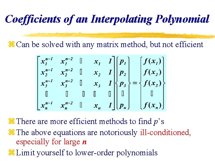
The coefficients $c_{1}, \dots, c_{n}$ are determined by the first $n$ values of the sequence, $x_{0}, x_{1}, \dots, x_{n - 1}$ , which we call the initial values. By setting $t = 0, 1, \dots, n - 1$ , we get a system of $n$ linear equations for the $n$ unknown coefficients $c_{i}$ :

⎩ ⎨ ⎧ x_{0} = c_{1} λ_{1}^{0} + c_{2} λ_{2}^{0} + \dots + c_{n} λ_{n}^{0} x_{1} = c_{1} λ_{1}^{1} + c_{2} λ_{2}^{1} + \dots + c_{n} λ_{n}^{1} ⋮ x_{n - 1} = c_{1} λ_{1}^{n - 1} + c_{2} λ_{2}^{n - 1} + \dots + c_{n} λ_{n}^{n - 1}

This can be written in matrix form:

1 λ_{1} λ_{1}^{2} ⋮ λ_{1}^{n - 1} 1 λ_{2} λ_{2}^{2} ⋮ λ_{2}^{n - 1} \dots \dots \dots ⋱ \dots 1 λ_{n} λ_{n}^{2} ⋮ λ_{n}^{n - 1} c_{1} c_{2} ⋮ c_{n} = x_{0} x_{1} ⋮ x_{n - 1}

The matrix on the left is a Vandermonde matrix. As long as the roots $λ_{i}$ are distinct, this matrix is invertible, which guarantees a unique set of coefficients $c_{i}$ for any given set of initial values $x_{k}$ .

This image shows the structure of the linear system we need to solve. The matrix is a Vandermonde matrix constructed from the characteristic roots $\lambda_i$. While this system can be solved directly, it can be numerically ill-conditioned. More importantly for our purposes, we want to understand its abstract structure.

2. Reframing with Polynomials

The structure of the system above hints at a deep connection to polynomials. Let's make this connection explicit.

Consider the space of polynomials in a complex variable $z$ with degree less than $n$ , denoted $P_{n - 1}$ . A basis for this space is the set of monomials: ${z^{0}, z^{1}, \dots, z^{n - 1}}$ .

Now, let's define a linear functional, $L$ , which maps polynomials from $P_{n - 1}$ to complex numbers. We can define this functional by specifying its action on our basis of monomials. Let's define it using our initial values:

$L (z^{k}) = x_{k} for k = 0, 1, \dots, n - 1$

Because $L$ is linear, its action on any polynomial $P (z) = \sum_{k = 0}^{n - 1} a_{k} z^{k}$ is uniquely determined:

$L (P) = L (\sum_{k = 0}^{n - 1} a_{k} z^{k}) = \sum_{k = 0}^{n - 1} a_{k} L (z^{k}) = \sum_{k = 0}^{n - 1} a_{k} x_{k}$

Now, let's look at the expression for $x_{t}$ again. The value $x_{t}$ is given by $x_{t} = \sum_{i = 1}^{n} c_{i} λ_{i}^{t}$ . This looks like the action of some operator on the monomial $z^{t}$ .

Let's see if our functional $L$ has a more revealing structure. From the system of equations in Section 1, we know that $x_{k} = \sum_{i = 1}^{n} c_{i} λ_{i}^{k}$ . Comparing this with our definition $L (z^{k}) = x_{k}$ , we find:

$L (z^{k}) = \sum_{i = 1}^{n} c_{i} λ_{i}^{k}$

This holds for $k = 0, \dots, n - 1$ . By linearity, for any polynomial $P (z) \in P_{n - 1}$ , we must have:

$L (P) = \sum_{i = 1}^{n} c_{i} P (λ_{i})$

This is a profound connection. It shows that the linear functional $L$ , which is entirely defined by the initial values $(x_{0}, \dots, x_{n - 1})$ , can also be expressed as a weighted sum of the polynomial's values at the characteristic roots. This form is known as a quadrature rule in numerical analysis.

3. The Interpolation Problem

We have now reframed our problem. The initial values $(x_{0}, \dots, x_{n - 1})$ are not just arbitrary numbers; they are the values of a specific linear functional $L$ on the basis of monomials ${z^{0}, \dots, z^{n - 1}}$ .

The problem of finding $x_{t}$ can now be stated as:

Given the values $L (z^{k}) = x_{k}$ for $k = 0, \dots, n - 1$ , what is the value of $L (z^{t})$ for $t \geq n$ ?

This is a classic problem of polynomial interpolation and extrapolation. We are given information about a function (our linear functional $L$ ) at a set of "points" (the monomials $z^{k}$ ) and we want to determine its value at another "point" ( $z^{t}$ ).

To better understand the concept of polynomial interpolation, let's review the standard formulation.

Polynomial interpolation

The following document, 'Polynomial interpolation' from NTNU, provides a concise and formal introduction to the topic. It will help solidify the core idea of finding a unique polynomial that passes through a given set of points.

Please read the section 'Interpolation problem' on page 1, and the section 'Existence and uniqueness of interpolation polynomials' on page 7. Focus on understanding the problem statement: given n+1 points, find a polynomial of degree n that passes through them. Note the theorem stating that such a polynomial is unique.

The resource you just read discusses finding a polynomial $p (x)$ that satisfies $p (x_{i}) = y_{i}$ for a given set of points $(x_{i}, y_{i})$ . Our problem is slightly different but deeply related. Instead of finding a polynomial, we are trying to determine the properties of a linear functional $L$ defined by its values on a basis of polynomials.

The key insight is that the structure of the difference equation solution imposes a very specific form on $L$ , namely $L (P) = \sum c_{i} P (λ_{i})$ . This structure is what allows us to "extrapolate" and find $L (z^{t}) = x_{t}$ .

The paper's authors leverage this reframing. The problem of maximizing $∣ x_{t} ∣$ over choices of roots $λ_{i}$ and initial values $x_{k}$ becomes a problem of maximizing $∣ L (z^{t}) ∣$ over choices of quadrature points $λ_{i}$ and the values $x_{k} = L (z^{k})$ . This moves the problem firmly into the realm of polynomial theory, which is the subject of the next lessons.

For a deeper dive into the mechanics of constructing such interpolating polynomials, the following video on Newton Interpolation is useful. While the paper's argument doesn't require these specific mechanics, understanding them reinforces the idea that the initial points uniquely determine the structure.

Newton Interpolation and Divided Differences

This video, 'Newton Interpolation and Divided Differences' by Dr. Will Wood, explains a powerful method for constructing an interpolating polynomial. It shows how the coefficients of the polynomial are systematically determined by the data points.

Please watch the following segments: Introduction (00:34 - 01:26): This introduces the form of the Newton polynomial. Calculating Coefficients (02:17 - 04:03): This shows how the first few coefficients are derived from the data points. Generalizing Divided Differences (05:37 - 06:42): This presents the recursive formula for all coefficients. Focus on the core idea: there is a systematic, unique way to determine the polynomial from the given points.

Conclusion

In this lesson, we have made a significant conceptual leap. We've shown that the task of finding a future term $x_{t}$ of a difference equation sequence, given its initial values $x_{0}, \dots, x_{n - 1}$ , is equivalent to a polynomial extrapolation problem.

Key Takeaways:

The initial values $(x_{0}, \dots, x_{n - 1})$ and characteristic roots $(λ_{1}, \dots, λ_{n})$ uniquely determine the coefficients $c_{i}$ in the general solution $x_{t} = \sum c_{i} λ_{i}^{t}$ via a Vandermonde system.
This relationship can be elegantly rephrased using a linear functional $L$ on the space of polynomials of degree less than $n$ .
The initial values define the functional by setting its values on the monomial basis: $L (z^{k}) = x_{k}$ .
The structure of the difference equation solution implies that this functional has the form of a quadrature rule: $L (P) = \sum_{i = 1}^{n} c_{i} P (λ_{i})$ .
Finding $x_{t}$ is equivalent to finding the value of this functional on the monomial $z^{t}$ , i.e., $L (z^{t})$ . This is the "interpolation problem over monomials" mentioned in the paper's abstract.

This new perspective is the launchpad for the rest of the paper's argument. In the next lesson, we will begin to apply this framework. We'll introduce some powerful tools from algebra—symmetric polynomials—and see how they relate to the coefficients of the characteristic polynomial, bringing us one step closer to solving the main optimization problem.