Optimizing Star-Schema Queries with EXPLAIN ANALYZE

Hello! Last lesson, you aligned sales and returns after aggregating each fact to the same reporting grain. That protected the answer from double counting. This lesson asks a different question: if a grain-safe report is slow, what physical change would help it without changing what the report means?

You will read a PostgreSQL execution plan, test an index against a realistic-sized example, and decide when partitioning or pre-aggregation is the better response. Allow about 50 minutes, including the short viewing and reading sections and the SQL investigation.

---

Read the work, not just the query

A star schema makes a business question straightforward to express, but its SQL can still require a large fact-table scan, a join, and an aggregate. EXPLAIN shows PostgreSQL’s proposed plan. EXPLAIN ANALYZE runs the query and adds observed row counts and timings. For a data-changing statement, that execution has real side effects; the queries in this lesson are read-only.

Watch these portions of A beginners guide to EXPLAIN ANALYZE by Michael Christofides on Tiger Data. The emphasis is on finding where work is spent rather than treating every sequential scan as a defect.

The PostgreSQL documentation gives the precise interpretation of the numbers. Read the indicated portions of “14.1. Using EXPLAIN” in the PostgreSQL 18 documentation (about 8 minutes).

Here is a compact example to interpret. The supplied image shows a PostgreSQL plan for an aggregate over a filtered sequential scan. It is not evidence of a slow query.

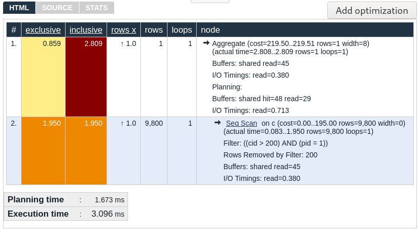
Read it from the scan upward. The scan examines roughly 10,000 rows and passes 9,800 to the aggregate. Its estimate of 9,800 output rows matches the observation. An index that finds 98% of this table would probably save little; PostgreSQL would still need most of the data. The scan’s approximately 1.950 ms is already included in the aggregate’s approximately 2.809 ms inclusive time. The image’s “exclusive” column attributes roughly 0.859 ms to work at the aggregate node itself. Do not add inclusive times or cumulative buffer counts across parent and child nodes.

When you inspect your own plans, start with four questions:

1. Where is time or buffer activity concentrated? A large fact scan, repeated join lookup, or sort can suggest different remedies.
2. How many rows enter and leave each node? rows describes a node’s output, not necessarily everything it examined. “Rows Removed by Filter” supplies another clue.
3. Were estimates reasonably close to actual rows? A substantial discrepancy may have influenced join or scan selection.
4. Does the proposed remedy eliminate meaningful work? An index is not a performance improvement merely because a plan uses it.

---

Establish a trustworthy baseline

The sales and returns tables from the previous lesson contain only a handful of rows. They are suitable for checking arithmetic, not for judging physical optimizations. PostgreSQL may correctly scan a tiny table even when an appropriate index exists. The following independent, disposable schema provides a larger sales fact and a small product dimension. Its fact grain is one generated sales line; each row’s sale_date and product_key describe that line.

Run this in a development database. Use a different schema name if lesson_perf already contains anything you need to keep.

CREATE SCHEMA lesson_perf;

CREATE TABLE lesson_perf.dim_product (
    product_key INTEGER PRIMARY KEY,
    category TEXT NOT NULL
);

INSERT INTO lesson_perf.dim_product (product_key, category)
SELECT
    product_key,
    'Group ' || lpad(((product_key - 1) / 10 + 1)::TEXT, 2, '0')
FROM generate_series(1, 200) AS g(product_key);

CREATE TABLE lesson_perf.fact_sales (
    sale_line_id BIGINT PRIMARY KEY,
    sale_date DATE NOT NULL,
    product_key INTEGER NOT NULL
        REFERENCES lesson_perf.dim_product (product_key),
    sales_amount NUMERIC(14, 2) NOT NULL
);

INSERT INTO lesson_perf.fact_sales (
    sale_line_id, sale_date, product_key, sales_amount
)
SELECT
    (day_date - DATE '2025-01-01') * 2000::BIGINT + line_no,
    day_date,
    line_no % 200 + 1,
    (line_no % 20 + 1)::NUMERIC(14, 2)
FROM generate_series(
    DATE '2025-01-01',
    DATE '2025-12-31',
    INTERVAL '1 day'
) AS days(day_date)
CROSS JOIN generate_series(1, 2000) AS lines(line_no);

ANALYZE lesson_perf.dim_product;
ANALYZE lesson_perf.fact_sales;

This creates 730,000 fact rows, evenly spread across dates and products. That makes the experiment repeatable, but its distribution may still differ greatly from a production sales workload. PostgreSQL’s “11.12. Examining Index Usage” explains why both collected statistics and representative data matter (about 3 minutes).

Now inspect a weekly, category-filtered star query before adding a fact-table date index:

EXPLAIN (ANALYZE, BUFFERS)
SELECT
    date_trunc('month', s.sale_date)::DATE AS month_start,
    p.category,
    SUM(s.sales_amount) AS gross_sales
FROM lesson_perf.fact_sales AS s
JOIN lesson_perf.dim_product AS p
  ON p.product_key = s.product_key
WHERE s.sale_date >= DATE '2025-07-01'
  AND s.sale_date <  DATE '2025-07-08'
  AND p.category = 'Group 01'
GROUP BY 1, 2
ORDER BY 1, 2;

The bounded predicate on s.sale_date is intentional: it identifies the fact-table rows needed for the report and is directly usable by a date-based access path. The result represents seven days’ sales for one category, grouped into its July reporting month. There are 14,000 sales lines in the selected week, of which 700 belong to Group 01.

Your exact plan and timings may differ. Locate the fact_sales scan, compare its estimated and actual output rows, and inspect Buffers: shared hit and read. A hit is a shared-buffer access; a read means PostgreSQL had to fetch a page into shared buffers. Buffer counts on a parent include its children, and repeated accesses need not represent distinct pages. Look at the execution time for the whole query as well as the nodes; planner cost units are not milliseconds.

---

Make an index earn its place

The weekly predicate narrows the date range to about 2% of this fact table. A B-tree index beginning with sale_date is therefore a reasonable candidate, not a promised win:

CREATE INDEX fact_sales_date_product_idx
    ON lesson_perf.fact_sales (sale_date, product_key);

ANALYZE lesson_perf.fact_sales;

Run the same EXPLAIN (ANALYZE, BUFFERS) query again. PostgreSQL might choose an index scan, a bitmap scan, or still choose a sequential scan. Compare the fact scan’s work, total execution time, and buffers before and after. Repeating each measurement under similar cache conditions is more informative than declaring victory from one timing.

The index’s leading date column supports this bounded date search. product_key may help with the join or filtering work, depending on the chosen plan; merely adding it does not guarantee that the category test will be performed inside the index. That category is stored in dim_product, not in this fact-table index. Conversely, a report scanning the whole year for all products may quite reasonably continue to use a sequential fact scan. Maintaining an index also costs storage and adds work to fact loads.

Choose indexing when the plan shows that a selective predicate or join can avoid enough row or page visits to justify those costs. If estimates are wildly inaccurate, check data and statistics before assuming an index is the missing component. If the query must read most fact rows to calculate its answer, an additional index may not address the expensive work.

---

When the date range calls for partitioning

Imagine that this fact contains several years of sales and reports routinely request one month. A date-range partitioning design can let PostgreSQL prune partitions outside the requested range. It also offers operational benefits when loading, retaining, or removing whole time periods. Partitioning is distinct from indexing: pruning avoids entire partitions, whereas an index finds rows within a relation or partition.

A plan for a suitable partitioned table might show an Append with only relevant child scans, or a scan naming just the relevant partition. If your predicate is only on an attribute of a joined date dimension, do not assume PostgreSQL can prune partitions keyed on the fact’s sale_date; verify the actual plan. Keeping the direct, bounded fact-date predicate makes the intended pruning test clear.

Partitioning is a design and migration decision, not an index-like command you can simply apply to the existing table. For illustration, a new parent could be declared with PARTITION BY RANGE (sale_date) and monthly partitions:

CREATE TABLE lesson_perf.fact_sales_partitioned (
    sale_line_id BIGINT NOT NULL,
    sale_date DATE NOT NULL,
    product_key INTEGER NOT NULL
        REFERENCES lesson_perf.dim_product (product_key),
    sales_amount NUMERIC(14, 2) NOT NULL,
    PRIMARY KEY (sale_date, sale_line_id)
) PARTITION BY RANGE (sale_date);

CREATE TABLE lesson_perf.fact_sales_2025_07
    PARTITION OF lesson_perf.fact_sales_partitioned
    FOR VALUES FROM ('2025-07-01') TO ('2025-08-01');

This illustrates one partition only; it is not yet a replacement for the full-year table. A PostgreSQL primary key on a partitioned table includes the partition key here so uniqueness can be enforced. In a production migration you would define the required partitions, move and validate the data, collect statistics, and compare plans and load behavior. Partitioning does not guarantee a faster seven-day query than the date index you just tested: even after pruning to July, that partition still contains many days. Too many small partitions can add planning and maintenance overhead.

Choose partitioning when plans show large amounts of irrelevant time-partition data can be excluded and the retention or load benefits justify it. Check for actual pruning and benchmark the complete workload, rather than judging the design by the presence of partition names in a plan.

---

When repeated summaries call for pre-aggregation

Now change the workload. Suppose a dashboard repeatedly asks for monthly sales by product category across a full year. The index on sale_date offers little help if virtually every fact row contributes. A precomputed summary can avoid repeating the fact scan, product join, and aggregation.

First, inspect the base query with EXPLAIN (ANALYZE, BUFFERS):

EXPLAIN (ANALYZE, BUFFERS)
SELECT
    date_trunc('month', s.sale_date)::DATE AS month_start,
    p.category,
    SUM(s.sales_amount) AS gross_sales
FROM lesson_perf.fact_sales AS s
JOIN lesson_perf.dim_product AS p
  ON p.product_key = s.product_key
WHERE s.sale_date >= DATE '2025-01-01'
  AND s.sale_date <  DATE '2026-01-01'
  AND p.category = 'Group 01'
GROUP BY 1, 2
ORDER BY 1, 2;

Build a materialized view whose declared reporting grain is one month and one category:

CREATE MATERIALIZED VIEW lesson_perf.monthly_category_sales AS
SELECT
    date_trunc('month', s.sale_date)::DATE AS month_start,
    p.category,
    SUM(s.sales_amount) AS gross_sales
FROM lesson_perf.fact_sales AS s
JOIN lesson_perf.dim_product AS p
  ON p.product_key = s.product_key
GROUP BY 1, 2;

ANALYZE lesson_perf.monthly_category_sales;

Then inspect the equivalent summary query:

EXPLAIN (ANALYZE, BUFFERS)
SELECT month_start, category, gross_sales
FROM lesson_perf.monthly_category_sales
WHERE month_start >= DATE '2025-01-01'
  AND month_start <  DATE '2026-01-01'
  AND category = 'Group 01'
ORDER BY month_start, category;

The materialized view contains only month/category groups, rather than 730,000 sales lines. Its query should need much less fact-level work—but confirm equal results, not just a faster plan. Compare the twelve output rows, their category, month, and amounts against the base query.

Pre-aggregation has a contract:

• It answers questions at its stored grain or a compatible coarser grain. It cannot recover individual sales lines or arbitrary daily figures.
• It must be refreshed when underlying sales or relevant category assignments change. The refresh has a cost and establishes a reporting-latency decision.
• Its measures must remain grain-safe. SUM(sales_amount) is appropriate here because each sale line contributes to exactly one month and one category. A rate or percentage would require its underlying numerator and denominator, not a sum of row-level percentages.
• In PostgreSQL, this query explicitly names the materialized view. Do not assume the optimizer will automatically substitute it for a query against the original fact and dimension tables.

This contrasts with the book’s DB2 examples of optimizer-directed aggregate navigation: the analytical idea transfers, but the rewrite behavior is database-specific. Your plan must confirm which relation PostgreSQL actually read.

---

Decide from the plan and the business question

The three remedies target different avoidable work:

Evidence and workload	Candidate to test	Principal trade-off
A selective fact-date or join lookup visits far more rows or pages than the answer needs	Index	Storage and slower writes; a broad scan may still be cheaper
A very large, time-organized fact repeatedly reads narrow date ranges	Date-range partitioning	Migration, partition management, and possible planning overhead
The same coarse summary repeatedly scans and joins many fact rows	Pre-aggregation	Refresh cost, data latency, and loss of finer detail in that summary

These are candidates, not mutually exclusive rules. A partitioned fact might also have local indexes; a dashboard might query a pre-aggregation built from that fact. Make the smallest change supported by observed work, then rerun the same SQL and compare correctness, execution time, row counts, and buffers. Include planning and refresh or load costs when those matter to the workload. EXPLAIN ANALYZE measures server-side execution, not the time to transmit a report to a BI client.

The overriding constraint is the one established in the previous lesson: optimization must not silently alter the reporting grain or duplicate a measure. If you eventually pre-aggregate both sales and returns, produce one summary per fact at identical conformed reporting headers, then align those summaries. A fast direct join of raw facts is still a wrong report.

---

Key takeaways

EXPLAIN ANALYZE lets you test an optimization against observed execution, rather than infer performance from schema shape or the mere existence of an index. Read plans from their scans upward; distinguish estimates from actual rows, inclusive node figures from exclusive work, and planner costs from milliseconds. Use realistic data and current statistics.

For a slow star query, test an index when a selective lookup can avoid work, partitioning when irrelevant date partitions can be pruned at useful scale, and pre-aggregation when a repeatedly requested coarse answer would otherwise recompute a large scan and join. In every case, validate the result as carefully as the runtime.

Next, you will review a draft dimensional model and use these performance observations alongside grain, key, hierarchy, additivity, and history checks to correct its design.