Why the Elementary Ratio Definition Fails for Continuous Conditioning

Hello. This course is narrowly about a familiar statistical expression whose usual notation conceals a genuine logical problem: what do we mean by $\mathbb{E}[Y\mid X=x]$ when $X$ is continuous and the event $\{X=x\}$ has probability zero?

You already know conditional means as objects used in prediction and regression. This lesson isolates why the elementary event-ratio definition works for discrete conditioning variables but cannot be carried over literally to a continuous covariate. The next lesson will replace the failed pointwise ratio with a condition about averages over regions of $X$-values.

---

The discrete formula, and the condition it quietly needs

For events $A$ and $B$, elementary conditional probability is defined by

$$\mathbb{P}(A\mid B)=\frac{\mathbb{P}(A\cap B)}{\mathbb{P}(B)},\mathbb{P}(B)>0.$$

The restriction is not a technical footnote. Dividing by $\mathbb{P}(B)$ normalizes the probability mass inside $B$, turning it into a new probability distribution. If there is no probability mass in $B$, there is nothing to normalize.

For a discrete $X$, conditioning on $X=x$ is simply conditioning on the event

$$\{X=x\}.$$

Provided $\mathbb{P}(X=x)>0$, the conditional mean can be written as

$$\mathbb{E}[Y\mid X=x]=\frac{\mathbb{E}\left[Y{1}_{\{X=x\}}\right]}{\mathbb{P}(X=x)}.$$

The numerator is the unconditional contribution to $Y$'s expectation from the group with $X=x$. Dividing by the group's probability gives its within-group average.

For example, suppose a credit-risk feature $X$ records a genuinely discrete rating band, and $Y$ is a loss outcome. If $20\%$ of accounts lie in a particular band, then the observed or modelled mean loss among that band has a straightforward population meaning. The event “rating band equals this one” contains a nonzero share of the population.

The key fact is therefore:

The ratio definition is a definition of conditioning on a positive-probability event.

---

A density height is not a probability

Now let $X$ be a continuously distributed variable, such as a measured yield, a log-price, a temperature, or a latent risk factor in an idealized model. If $X$ has density $f_X$, then the probability of an interval is an area:

$$\mathbb{P}(a<X<b)={\int }_a^b{f}_X(t)dt.$$

At one exact value $x$, the relevant set has no width, so its area is zero:

$$\mathbb{P}(X=x)={\int }_{\{x\}}{f}_X(t)dt=0.$$

This remains true even if the density is high at $x$. The number $f_X(x)$ is a density, measured in “probability per unit of $X$,” not a probability.

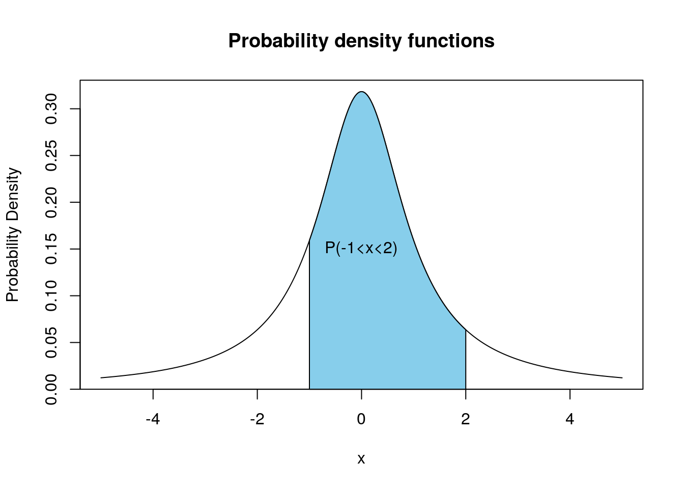
This is a common source of notational misdirection. A density plot can make a value near the mode look “likely,” which is useful informal language. But the precise statement is that values in a small neighbourhood of the mode have relatively high probability. It is not that $X$ has a positive probability of equalling the mode exactly.

Consequently, the discrete formula becomes

$$\frac{\mathbb{E}\left[Y{1}_{\{X=x\}}\right]}{\mathbb{P}(X=x)}=\frac{0}{0}.$$

Why is the numerator also zero? Since $\{X=x\}$ is a null event, its indicator satisfies

$$1_{\{X=x\}}=0\text{almost surely}.$$

For integrable $Y$, this implies

$$\mathbb{E}\left[Y{1}_{\{X=x\}}\right]=0.$$

The failure is therefore not “a very small number divided by another very small number.” It is an undefined $0/0$ expression.

---

Zero probability does not mean impossible

In elementary presentations, “probability zero” is sometimes casually glossed as “impossible.” That is safe only in some finite or discrete settings. It is misleading here.

If a continuously distributed $X$ is realised, it takes some exact value. Yet for every fixed value selected in advance,

$$\mathbb{P}(X=x)=0.$$

There is no contradiction. Probability measures quantify the probability of sets of possible outcomes. A single point is too small, geometrically, to receive positive mass under a continuous distribution.

Think of an idealized observation of a continuously varying financial quantity. The model may assign probability zero to the pre-specified statement “the value will be exactly $x$.” Once an observation occurs, however, it has a particular realised value. The issue is not whether one can observe a number; it is whether the elementary probability law identifies a conditional distribution on that exact null event.

In real data, recorded values are rounded and have finite precision, so “$X=2000$” often actually means “$X$ lies in a narrow reporting bin around 2000.” That event can have positive probability. But the theoretical continuous model deliberately idealizes away the bins, and then demands an account of what the pointwise notation means.

---

Why this is more than a division-by-zero annoyance

One might try to dismiss the problem: surely we can just define whatever value seems reasonable at $x$. But that response exposes the deeper issue.

Suppose some function $m$ is accepted as the conditional-mean function. Change its value at one point $x_0$:

$$\tilde{m}(x)=\{\begin{array}{ll}m(x),& x\ne x_0,\\ m(x_0)+1000,& x=x_0.\end{array}$$

If $X$ is continuous, then

$$\mathbb{P}(X=x_0)=0.$$

So $m(X)$ and $\tilde{m}(X)$ differ only on an event of probability zero. They have the same expectation, the same mean squared prediction error, and the same implications for any population average. No calculation based solely on the joint probability distribution of $(X,Y)$ can distinguish them.

This tells us exactly what an event-ratio formula could not tell us:

The joint distribution does not, by itself, determine a conditional mean at every individual zero-probability point.

This matters for the eventual interpretation of regression. A regression function such as

$$m(x)=\mathbb{E}[Y\mid X=x]$$

is meant to summarize the mean outcome at covariate value $x$. In a continuous model, its population role is fundamentally about how it behaves over sets of $X$-values carrying probability mass, not initially about an independently determined answer at each isolated coordinate.

Later, under useful regularity conditions, we often choose a natural pointwise representative: for instance, a continuous version of the conditional mean, or one constructed from a conditional density. That is a valuable choice, often exactly the one intended in applied work. But it is an additional construction, not the elementary ratio formula magically revived.

---

The tempting neighbourhood repair

There is a sensible intuition behind the notation “given $X=x$.” Instead of conditioning on the point, condition on a shrinking interval around it:

$$\mathbb{E}[Y\mid x-h<X<x+h].$$

For each fixed $h>0$ for which the interval has positive probability, this is an ordinary conditional expectation:

$$\mathbb{E}[Y\mid x-h<X<x+h]=\frac{\mathbb{E}\left[Y{1}_{\{x-h<X<x+h\}}\right]}{\mathbb{P}(x-h<X<x+h)}.$$

Under sufficiently well-behaved density and smoothness assumptions, these local averages can converge as $h$ shrinks. The limiting value is then a compelling candidate for the conditional mean at $x$.

This local-average picture underlies the practical intuition behind nonparametric regression: data close to a covariate value are used to estimate the mean response there. Parametric regression makes stronger structural assumptions, such as linearity, to borrow information across such neighbourhoods.

But this limit is not a universal elementary definition:

• it presupposes that appropriate shrinking neighbourhoods have positive probability;
• the limit may fail to exist at irregular points;
• even when a conditional object is well-defined in the measure-theoretic sense, its value can remain undetermined on a set of $X$-values of probability zero.

Thus neighbourhood conditioning motivates the answer, but does not supply the general foundation.

---

What has failed, precisely

The notation $\mathbb{E}[Y\mid X=x]$ invites the discrete formula

$$\frac{\mathbb{E}[Y{1}_{\{X=x\}}]}{\mathbb{P}(X=x)}.$$

For continuously distributed $X$, both terms are zero. The formula is undefined, and the joint probability law cannot identify a unique answer at one isolated $x$. A density value at $x$ does not solve the problem, because density is not point probability.

The right replacement will deliberately stop treating $\{X=x\}$ as the primitive conditioning event. Instead, it will characterize a function $m(X)$ by requiring it to reproduce $Y$'s averages over every measurable region of the $X$-space. That regional requirement is the bridge from familiar conditional means to the Radon–Nikodym construction that eventually grounds the notation $\mathbb{E}[Y\mid X=x]$.