MLE for Cross-Entropy and MSE Loss Functions

Welcome to the final lesson of our foundational module on neural networks. In our previous discussions, we established that neural networks are compositions of affine transformations and non-linearities, and we proved, via the Universal Approximation Theorem, that even a simple network is theoretically capable of representing any continuous function.

This is a powerful guarantee of expressivity, but it doesn't tell us how to find the specific network parameters that solve a given problem. To do that, we need to transition from theory to practice—we need a way to train the network. Training is an optimization problem, and at the heart of any optimization problem is an objective function—a way to measure how well our model is currently performing. In machine learning, we call this the loss function.

Today, we will derive the two most important loss functions in all of machine learning—Mean Squared Error (MSE) for regression and Cross-Entropy for classification. Instead of just presenting them as formulas to be memorized, we will derive them from a single, powerful statistical principle: Maximum Likelihood Estimation (MLE). This will provide a deep, probabilistic justification for why these specific functions are so fundamental to training neural networks and other machine learning models.

The Principle of Maximum Likelihood Estimation (MLE)

Before we can derive our loss functions, we must first understand the principle they are built upon. Maximum Likelihood Estimation is a general method for estimating the parameters of a statistical model. The core idea is intuitive: we should choose the parameters that make our observed data the most probable.

Imagine you have a set of data points, and you are trying to find a probability distribution that best describes them. You could try various distributions, each defined by a set of parameters (like the mean and variance of a Gaussian). For each candidate distribution, you can calculate the probability, or "likelihood," of having observed your specific data. MLE simply states that the best set of parameters is the one that maximizes this likelihood.

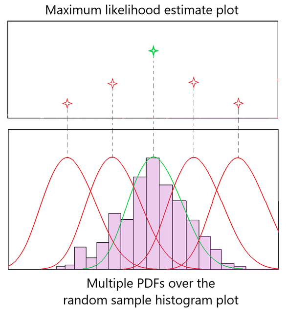
This idea is formalized in the likelihood function.

To summarize the key points:

1. Likelihood Function: Given a dataset $D=\{y^{(1)},...,y^{(N)}\}$ and a model parameterized by $\theta$, the likelihood, assuming data is independent and identically distributed (i.i.d.), is: $$L(\theta ;D)=p(D|\theta )=\prod _{i=1}^{N}p(y^{(i)}|\theta )$$
2. Log-Likelihood: To make optimization tractable, we work with the log-likelihood: $$\ell (\theta ;D)=\log L(\theta ;D)=\sum _{i=1}^N\log p(y^{(i)}|\theta )$$
3. The Goal of MLE: We want to find the parameters ${\hat{\theta }}_{\text{MLE}}$ that maximize this function: $${\hat{\theta }}_{\text{MLE}}=\arg \underset{\theta }{\max }\ell (\theta ;D)$$
4. Connection to Minimization: Since standard optimization algorithms like gradient descent are framed as minimization problems, we typically minimize the negative log-likelihood (NLL), which is an equivalent problem: $${\hat{\theta }}_{\text{MLE}}=\arg \underset{\theta }{\min }J(\theta )\text{where}J(\theta )=-\ell (\theta ;D)$$

This final expression, $J(\theta )$, is our loss function. The process of minimizing the NLL is the process of training our model.

Deriving Mean Squared Error (MSE) for Regression

Let's apply this principle to a regression problem. Our goal is to train a neural network, $f(x;\theta )$, to predict a continuous target variable $y$.

The crucial step in MLE is to make a probabilistic assumption about how the data is generated. For regression, the standard assumption is that the target $y$ is not perfectly determined by the input $x$, but includes some zero-mean Gaussian noise. In other words, we assume the target $y^{(i)}$ is drawn from a Normal distribution whose mean is the network's output $f(x^{(i)};\theta )$ and whose variance is some fixed ${\sigma }^2$.

Assumption: $p(y^{(i)}|x^{(i)};\theta )=\mathcal{N}(y^{(i)}|f(x^{(i)};\theta ),{\sigma }^2)$

The probability density function for a single data point $(x^{(i)},y^{(i)})$ is therefore:

$$p(y^{(i)}|x^{(i)};\theta )=\frac{1}{\sqrt{2\pi {\sigma }^2}}\exp \left(-\frac{(y^{(i)}-f(x^{(i)};\theta ){)}^2}{2{\sigma }^2}\right)$$

Before we derive the loss function from this, let's watch a video that demonstrates the general procedure for finding the MLE of a Gaussian distribution's parameters. This will solidify the mechanics before we apply them to our specific neural network case.

Now, let's apply this exact same logic to our regression problem. We form the log-likelihood for the entire dataset $D=\{(x^{(1)},y^{(1)}),...,(x^{(N)},y^{(N)})\}$:

$$\ell (\theta ,\sigma )=\sum _{i=1}^N\log p(y^{(i)}|x^{(i)};\theta )=\sum _{i=1}^N\log \left(\frac{1}{\sqrt{2\pi {\sigma }^2}}\exp \left(-\frac{(y^{(i)}-f(x^{(i)};\theta ){)}^2}{2{\sigma }^2}\right)\right)$$

Using the properties of logarithms, we can simplify this expression:

$$\ell (\theta ,\sigma )=\sum _{i=1}^N\left[\log \left(\frac{1}{\sqrt{2\pi {\sigma }^2}}\right)-\frac{(y^{(i)}-f(x^{(i)};\theta ){)}^2}{2{\sigma }^2}\right]$$ $$\ell (\theta ,\sigma )=-N\log (\sqrt{2\pi }\sigma )-\frac{1}{2{\sigma }^2}\sum _{i=1}^N(y^{(i)}-f(x^{(i)};\theta ){)}^2$$

Our goal is to find the network parameters $\theta$ that maximize this log-likelihood. Notice that the first term, $-N\log (\sqrt{2\pi }\sigma )$, does not depend on $\theta$. Therefore, to maximize $\ell (\theta ,\sigma )$ with respect to $\theta$, we only need to maximize the second term.

Maximizing $-\frac{1}{2{\sigma }^2}{\sum }_{i=1}^N(y^{(i)}-f(x^{(i)};\theta ){)}^2$ is equivalent to minimizing its negation:

$${\hat{\theta }}_{\text{MLE}}=\arg \underset{\theta }{\max }\left[-\frac{1}{2{\sigma }^2}\sum _{i=1}^N(y^{(i)}-f(x^{(i)};\theta ){)}^2\right]=\arg \underset{\theta }{\min }\left[\frac{1}{2{\sigma }^2}\sum _{i=1}^N(y^{(i)}-f(x^{(i)};\theta ){)}^2\right]$$

Since $2{\sigma }^2$ is a positive constant with respect to $\theta$, we can drop it from the optimization. We are left with:

$${\hat{\theta }}_{\text{MLE}}=\arg \underset{\theta }{\min }\sum _{i=1}^N(y^{(i)}-f(x^{(i)};\theta ){)}^2$$

This is exactly the Sum of Squared Errors. If we average it over the dataset by dividing by $N$, we arrive at the familiar Mean Squared Error (MSE) loss function. Thus, we have shown that minimizing MSE is equivalent to performing Maximum Likelihood Estimation under the assumption of Gaussian noise.

Deriving Cross-Entropy for Classification

Now, let's turn to classification. Here, our network's output $\hat{y}$ is a probability (or a vector of probabilities for multi-class problems), and our true label $y$ is a class index.

The key assumption for classification is that the true label is drawn from a discrete probability distribution whose parameters are given by the network's output.

• For binary classification ($y\in \{0,1\}$), we assume $y$ follows a Bernoulli distribution.
• For multi-class classification ($y$ is a one-hot vector), we assume $y$ follows a Categorical distribution.

The CMU notes you read earlier have a fantastic section that performs this derivation explicitly for logistic regression. Since a neural network's final layer for classification is typically a logistic (sigmoid) or softmax function, this derivation applies directly.

Let's recap the results from that reading.

Binary Cross-Entropy:

• Assumption: $y\sim \text{Bernoulli}(\hat{y})$, where $\hat{y}=f(x;\theta )$ is the network's output probability for class 1.
• Likelihood (one point): $p(y|\hat{y})={\hat{y}}^y(1-\hat{y}{)}^{1-y}$
• Negative Log-Likelihood (Loss): $$J(\theta )=-\sum _{i=1}^N\left[y^{(i)}\log ({\hat{y}}^{(i)})+(1-y^{(i)})\log (1-{\hat{y}}^{(i)})\right]$$ This is precisely the binary cross-entropy loss.

Categorical Cross-Entropy:

• Assumption: $y\sim \text{Categorical}(\hat{y})$, where $\hat{y}$ is the vector of $K$ probabilities from the network's softmax output.
• Likelihood (one point): $p(y|\hat{y})={\prod }_{k=1}^K({\hat{y}}_k{)}^{y_k}$
• Negative Log-Likelihood (Loss): $$J(\theta )=-\sum _{i=1}^N\sum _{k=1}^K{y}_k^{(i)}\log ({\hat{y}}_k^{(i)})$$ This is the categorical cross-entropy loss.

The term "cross-entropy" itself comes from information theory, where it measures the difference between two probability distributions (the true distribution defined by $y$ and the predicted distribution defined by $\hat{y}$). Our derivation shows that minimizing this information-theoretic quantity is equivalent to maximizing the likelihood of the observed data.

Conclusion

In this lesson, we have forged a critical link between the abstract principles of statistics and the practical machinery of training neural networks. We've moved beyond simply stating loss functions and have derived them from first principles.

Key Takeaways:

• Maximum Likelihood Estimation (MLE) provides a foundational principle for deriving objective functions. The goal is to find model parameters that maximize the probability of the observed data.
• In practice, we minimize the negative log-likelihood (NLL), which is numerically stable, mathematically convenient, and aligns with standard gradient-based optimization.
• Minimizing Mean Squared Error (MSE) in regression is equivalent to performing MLE under the assumption that the data contains Gaussian noise.
• Minimizing Cross-Entropy in classification is equivalent to performing MLE under the assumption that the class labels are generated from a Bernoulli or Categorical distribution parameterized by the network's outputs.

This concludes our first module. We now have all the conceptual components of a feedforward neural network: we know its architecture (Lesson 3), we know it is a powerful approximator (Lesson 6), and we now have a principled way to define the objective function we want to optimize (this lesson).

The only remaining question is how to perform this optimization. How do we efficiently calculate the gradients of this loss function with respect to the millions of parameters in a deep network? The answer lies in the elegant algorithm that powers all of modern deep learning: backpropagation. This will be the subject of our first lesson in the next module.