Perfect Competition: Short-Run Profit/Loss

Introduction

Welcome to the next lesson in our exploration of firm behavior! In our last session, we established the universal profit-maximization rule: firms produce at the quantity where Marginal Revenue equals Marginal Cost (MR = MC). This rule is the analytical engine we'll use to understand how firms make decisions.

So far, we've treated the firm in isolation. But in reality, firms operate within specific market environments, or market structures, which dictate the nature of competition and influence their pricing power. In this module, we will analyze four main structures: perfect competition, monopoly, monopolistic competition, and oligopoly.

Today, we begin with the most foundational model: perfect competition. Our goal is to identify the characteristics that define this market structure and then use our graphical tools—combining the cost curves from Module 4 with the MR=MC rule—to determine if a competitive firm is making a profit or a loss in the short run.

1. The World of Perfect Competition

What makes a market "perfectly competitive"? It's an idealized model, but it provides a crucial benchmark for understanding all other market structures. It is defined by a specific set of characteristics.

To get a quick overview of these features, let's start with a video.

As you just saw, a market is perfectly competitive if it meets these conditions:

1. Many Buyers and Sellers: There are so many firms and consumers that no single one can influence the market price. Each firm is a tiny player in the overall market.
2. Homogeneous Products: All firms sell an identical, undifferentiated product. Think of commodities like #2 yellow corn or raw milk. From a buyer's perspective, the product from one firm is a perfect substitute for the product from any other firm.
3. No Barriers to Entry or Exit: Firms can freely and easily enter the market if they see an opportunity for profit, and leave if they are making losses.
4. Perfect Information: All buyers and sellers have complete information about prices, technology, and product quality.

The Firm as a Price Taker

The direct consequence of these assumptions is that a perfectly competitive firm is a price taker. It has no power to set its own price; it must accept the price determined by the forces of supply and demand in the overall market.

Why? If a single farmer tried to sell their corn for even a few cents more than the market price, rational buyers with perfect information would simply buy from one of the countless other farmers selling the identical product at the market price. Conversely, there's no reason to sell for less, as the firm can sell all it wants at the prevailing market price.

This leads to a crucial graphical insight:

• The market has a standard downward-sloping demand curve and an upward-sloping supply curve, which together determine the equilibrium price, $P_{market}$.
• The individual firm faces a perfectly elastic (horizontal) demand curve at this exact market price.

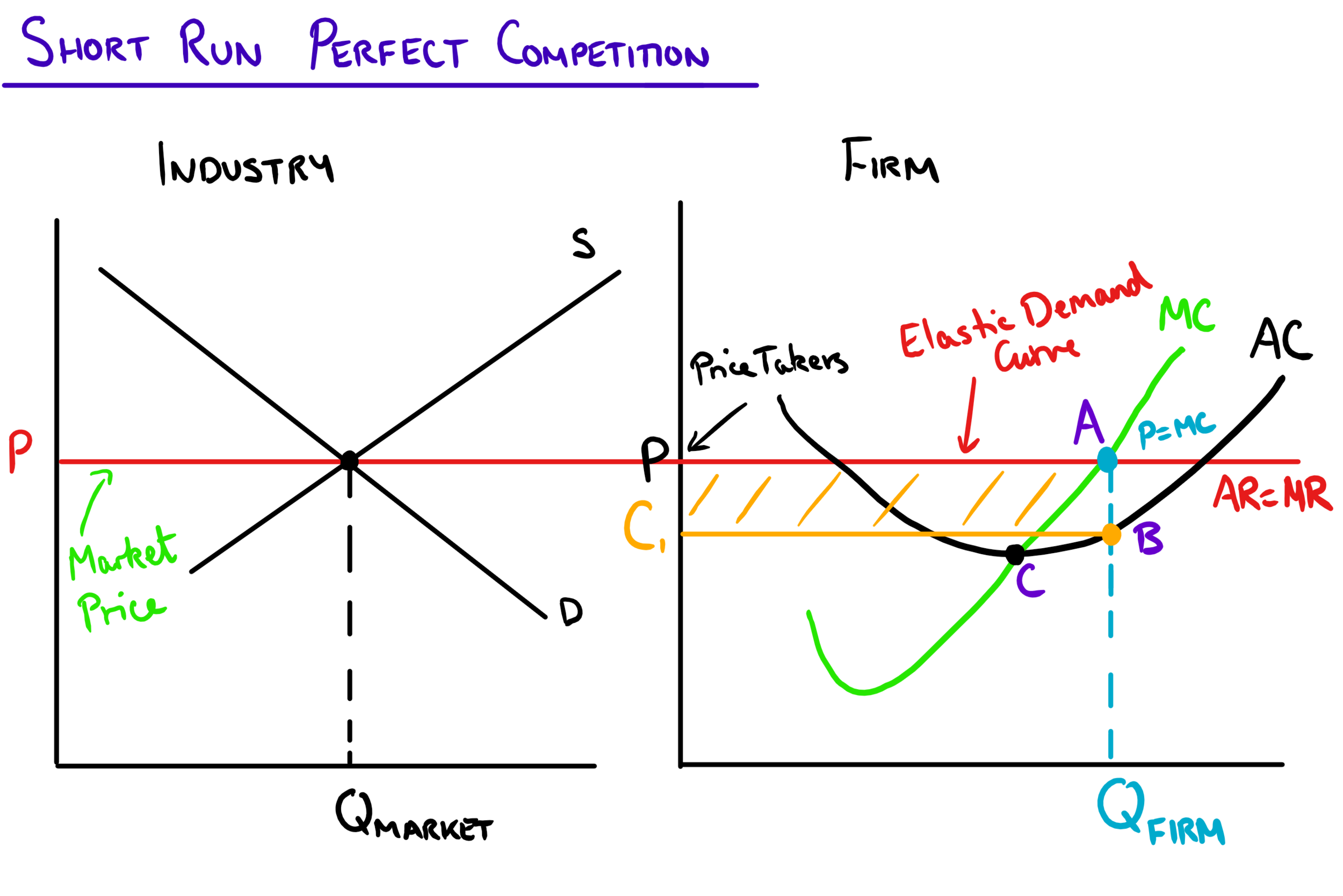
Because the firm receives the same price for every single unit it sells, that price is also its marginal revenue (MR) and its average revenue (AR). This gives rise to a famous mnemonic: for a perfectly competitive firm, the demand curve is Mr. DARP (Marginal Revenue = Demand = Average Revenue = Price).

2. Determining Short-Run Profit or Loss

Now we can combine everything we've learned. We will use the firm's cost curves (MC, ATC) and its new horizontal revenue curve (D = MR = AR = P) to analyze its profitability. The process is a straightforward application of the MR=MC rule.

The 3-Step Method:

1. Find Quantity (q*): Apply the profit-maximization rule. Find the quantity where MR = MC. Graphically, this is the intersection of the horizontal price line and the marginal cost curve.
2. Find Total Revenue (TR) and Total Cost (TC): At quantity q*, find the price (P) and the average total cost (ATC).
   • Total Revenue = $P\times q\text{*}$
   • Total Cost = $ATC\times q\text{*}$
3. Calculate Profit or Loss: Compare the price and the average total cost at the profit-maximizing quantity.
   • Profit: If $P>ATC$, the firm is making a positive economic profit.
   • Loss: If $P<ATC$, the firm is suffering an economic loss.
   • Break-Even: If $P=ATC$, the firm is earning zero economic profit.

Let's see this process in action.

Scenario 1: Making a Profit (P > ATC)

When the market price is high enough, a firm can earn positive economic profits. The following video segment demonstrates how to draw this scenario.

Scenario 2: Incurring a Loss (P < ATC)

If the market price falls, the firm might face a situation where it cannot cover all its costs. This results in an economic loss.

It's important to note that making a loss doesn't automatically mean the firm will shut down. As long as the price is high enough to cover its average variable costs, the firm is better off producing and losing some money than shutting down and losing all its fixed costs. We will explore this "shutdown rule" in more detail later.

Putting It All Together

The following reading provides a great summary of all three scenarios—profit, loss, and the break-even point—with clear, static diagrams that you can study at your own pace.

To consolidate your understanding, the image below shows all three short-run possibilities for a perfectly competitive firm side-by-side.

Conclusion

In this lesson, we have taken a major step in applying economic theory to a specific market context. We defined the ideal model of perfect competition and understood its profound implication: firms are price takers with perfectly elastic demand curves.

Here are the key takeaways:

• Characteristics of Perfect Competition: Many firms, identical products, no barriers to entry, and perfect information.
• Price Taker: A competitive firm must accept the market price, meaning its demand curve is horizontal. For this firm, Price = Average Revenue = Marginal Revenue.
• Short-Run Profit/Loss Analysis: To determine profitability, you first find the profit-maximizing quantity where MR = MC, and then at that quantity, you compare the Price (P) to the Average Total Cost (ATC).

The existence of profits or losses is a temporary, short-run situation. These outcomes send powerful signals to the rest of the market. Profits attract new firms to enter, while losses push existing firms to exit. In our next lesson, we will explore how this process of entry and exit drives perfectly competitive markets toward a long-run equilibrium where economic profits are zero.