Recommended resources
The freely available resources this lesson will direct you to.
Hello! This module is about turning rows into useful summaries: first by grouping and aggregating, then by filtering groups and calculating more specialized metrics. In this lesson, you’ll learn to decide what one output row represents—the result’s grain—and use GROUP BY with aggregate functions to produce that summary.
The central habit is to state the grain before writing the query. “Total sales” asks for one row overall; “total sales per category” asks for one row per category. Those are different questions, even when they use the same table and the same SUM() function.
Decide what one result row means
Suppose a sales table contains one row per sale:
| sale_id | category | channel | amount |
|---|---|---|---|
| 101 | books | web | 20 |
| 102 | books | web | 30 |
| 103 | books | store | 10 |
| 104 | games | web | 40 |
| 105 | games | store | 15 |
| 106 | games | store | NULL |
| 107 | games | web | 5 |
| 108 | books | store | 25 |
At the table’s grain, each row describes a sale. If the question asks for the total amount across all sales, an aggregate alone produces one summary row:
SELECT
    COUNT(*) AS sale_rows,
    SUM(amount) AS total_amount
FROM sales;
The result is 8 sale rows and a total amount of 145. There is no GROUP BY because the requested grain is the entire table.
Now change the question to “What is the total amount per category?” The desired grain is one row per category. GROUP BY category collects rows sharing a category value, and SUM(amount) calculates a result within each collection.
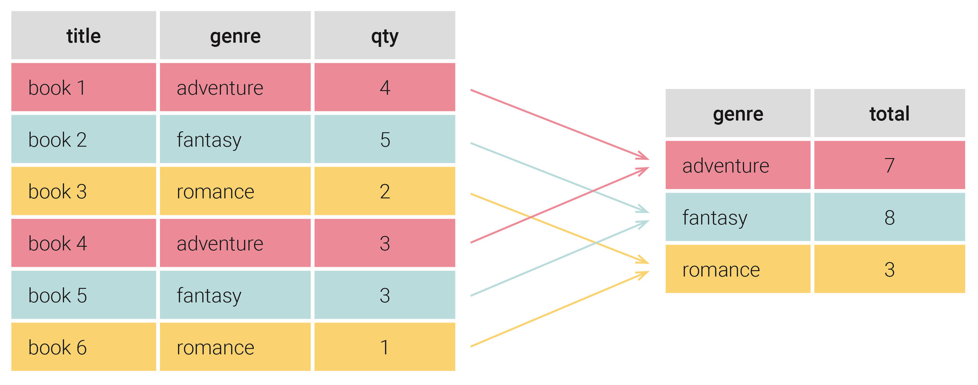
The image uses books and genres; the same principle applies to sales and categories. Notice that grouping does not merely put similar rows next to each other. It produces a summary at a new grain.
Watch “MySQL: GROUP BY” from Bro Code for a short demonstration of how changing the grouping column changes the question a query answers. The basic GROUP BY and aggregate syntax shown here also applies to PostgreSQL.
Watch the introduction for the purpose of grouping. Then watch daily summaries, where the presenter groups transactions by date and applies several aggregate functions. Continue with customer summaries: focus on how grouping the same transactions by customer instead produces a different kind of result.
Calculate metrics within each group
Here is the sales query at one row per category:
SELECT
    category,
    COUNT(*) AS sale_rows,
    COUNT(amount) AS recorded_amounts,
    SUM(amount) AS total_amount,
    AVG(amount) AS average_amount
FROM sales
GROUP BY category
ORDER BY category;
| category | sale_rows | recorded_amounts | total_amount | average_amount |
|---|---|---|---|---|
| books | 4 | 4 | 85 | 21.25 |
| games | 4 | 3 | 60 | 20 |
Read the first result row as a sentence: “For books, there are four sale rows; their amounts total 85 and average 21.25.” The second row describes games. ORDER BY category makes the output predictable to read; it does not determine the groups.
Two counts appear because they answer different questions. COUNT(*) counts rows, including sale 106. COUNT(amount) counts rows whose amount is not NULL, so it excludes that sale. SUM(amount) and AVG(amount) also ignore NULL amounts. Consequently, the games average is , not . An unknown amount is not the same as an amount of zero.
The other common aggregates are MIN() and MAX(). For example, this query finds the smallest and largest recorded sale amounts in each category:
SELECT
    category,
    MIN(amount) AS smallest_amount,
    MAX(amount) AS largest_amount
FROM sales
GROUP BY category
ORDER BY category;
For books, the smallest and largest amounts are 10 and 30; for games, they are 5 and 40. Like SUM() and AVG(), these functions ignore NULL inputs. If a group has no non-NULL amounts, COUNT(amount) returns zero, while these amount-based aggregates return NULL.
SQL Lesson 10: Queries with aggregates (Pt. 1)
Read SQLBolt’s explanation to consolidate what each common aggregate measures and why GROUP BY changes an aggregate from a whole-table calculation to a per-group calculation.
Under “Common aggregate functions,” read the function table, paying particular attention to the distinction between counting rows and counting non-NULL column values. Then, under “Grouped aggregate functions,” read the grouping explanation, including its query pattern. Stop before the “Exercise” heading.
Set a more detailed grain with multiple columns
A category total cannot tell you whether its sales came through the web or a store. To answer “What is the total amount per category and channel?”, both columns must define the groups:
SELECT
    category,
    channel,
    COUNT(*) AS sale_rows,
    SUM(amount) AS total_amount
FROM sales
GROUP BY category, channel
ORDER BY category, channel;
| category | channel | sale_rows | total_amount |
|---|---|---|---|
| books | store | 2 | 35 |
| books | web | 2 | 50 |
| games | store | 2 | 15 |
| games | web | 2 | 45 |
Each output row now represents a distinct category–channel combination present in the data. The games–store group has two sale rows but totals 15: one of its amounts is NULL. Adding channel made the result more detailed than the category-only summary; it did not change what SUM(amount) means.
This leads to a useful rule for constructing queries: put the columns that define the requested grain in GROUP BY; put the measurements you want to summarize inside aggregate functions. In these examples, category and sometimes channel identify a result row, while amount supplies values to calculate.
Selecting sale_id in the category-level query without aggregating it would break that logic: a category contains several sale IDs, so which single ID could the result display? Standard SQL generally rejects such a selection. Grouping by sale_id merely to make the query run is not a fix—it changes the grain back toward one row per sale and loses the requested category summary.
Keep the question attached to the result
When checking an aggregate query, read its output grain aloud: “one row overall,” “one row per category,” or “one row per category and channel.” Then check that each metric means what its label claims. In particular, distinguish a count of rows from a count of recorded values, and remember that AVG() uses non-NULL values rather than every row in the group.
You can now summarize a table with COUNT(), SUM(), AVG(), MIN(), and MAX() at a chosen grain. The next lesson adds filtering: how to decide whether a condition should remove individual rows before aggregation or remove entire groups after their metrics have been calculated.