Big-O Notation: Analyzing Algorithm Complexity

1. What is Big-O and Why Does It Matter?

At its core, Big-O notation isn't about measuring the exact runtime of a program in seconds. Instead, it describes how the runtime or memory usage of an algorithm scales as the input size (n) grows. It provides a high-level understanding of an algorithm's efficiency, focusing on its growth rate.

To get a strong conceptual foundation, let's start with a video that explains the core ideas.

As the video highlights, when analyzing complexity, we're typically interested in the worst-case scenario. This gives us an upper bound on the performance, ensuring we're prepared for the most demanding situations.

To solidify these rules of simplification, please read the following short text.

The key takeaways are:

• Focus on Growth: We care about how performance changes as the input n gets very large.
• Worst-Case Analysis: We usually analyze the upper bound of performance.
• Drop Constants: O(2n) is simplified to O(n).
• Drop Lower-Order Terms: O(n² + n) is simplified to O(n²).

2. The Hierarchy of Complexity Classes

Algorithms are categorized into different complexity classes. Understanding this hierarchy is crucial because it allows you to quickly judge the feasibility of a potential solution. An algorithm that is O(n²) might be fine for 100 items, but it will be disastrous for a million.

The following video walks through the most common complexity classes you'll encounter, from fastest to slowest.

Here is a summary of the common classes, from best to worst:

• O(1) - Constant: The runtime is independent of the input size. (e.g., accessing an array element by index).
• O(log n) - Logarithmic: The runtime grows very slowly. Common in algorithms that divide the problem in half at each step (e.g., binary search).
• O(n) - Linear: The runtime grows proportionally to the input size. (e.g., iterating through a list).
• O(n log n) - Linearithmic: A very common complexity for efficient sorting algorithms (e.g., Merge Sort, Quicksort).
• O(n²) - Quadratic: The runtime grows exponentially. Often involves nested loops over the same input (e.g., bubble sort, checking all pairs in a list).
• O(2ⁿ) - Exponential: The runtime doubles with each new element. Often seen in recursive solutions that solve a problem of size n by making two recursive calls for size n-1 (e.g., naive recursive Fibonacci).
• O(n!) - Factorial: The runtime grows extremely quickly. Typically involves generating all permutations of a set.

This chart provides a great visual reference for these classes and the types of algorithms they correspond to.

To see just how dramatic the difference is, the "Complete guide to big-O" article has a powerful graph and table in section 1.1.3 How big-O classes compare to one another. It shows that for an input of just n=60, an O(2ⁿ) algorithm would take centuries on a fast machine!

3. From Theory to Practice: Analyzing Code

Now, let's apply these concepts to actual Python code. The goal is to develop the ability to look at a function and quickly determine its time and space complexity.

Time Complexity is the measure of how many operations an algorithm performs.
Space Complexity is the measure of how much extra memory (or auxiliary space) an algorithm needs, not including the space taken up by the input itself.

This next video is fantastic because it's purely focused on walking through Python code snippets and analyzing them.

4. Big-O in the Python Ecosystem and Trade-offs

A key skill for a Python developer is knowing the complexity of built-in operations. Choosing the right data structure for the job often comes down to understanding these performance characteristics. Using a list when you need fast lookups can lead to an O(n) operation where a dict or set would have given you O(1).

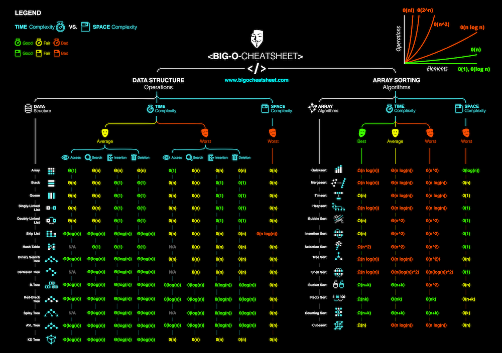
The Ultimate Cheat Sheet

The following image is an indispensable resource. Many engineers print it out or keep it handy. It summarizes the time and space complexity for all major data structures and sorting algorithms. We will cover all of these topics in this course, so this will be your companion throughout.

Conclusion

In this lesson, we've laid the essential groundwork for our entire course. You've learned what Big-O notation is and, more importantly, why it's the primary tool for reasoning about algorithm efficiency.

Key Takeaways:

• Big-O measures scalability: It describes the growth rate of an algorithm's time or space requirements as the input size increases.
• Simplification is key: We focus on the dominant term, dropping constants and lower-order terms to analyze the overall trend.
• Hierarchy matters: The difference between O(n log n) and O(n²) is not just academic; it determines whether an application can handle real-world scale.
• Analysis is a practical skill: You can determine complexity by examining code structures like loops (multiplicative when nested) and recursion (depends on the number of branches).
• Know your tools: Understanding the Big-O of Python's built-in data types is critical for writing performant code.

Preview of the Next Lesson

Now that you have the tools to analyze complexity, we'll immediately put them to use. In the next lesson, we will dive into our first data structure: the dynamic array, which you know as Python's list. We'll dissect its internal workings and analyze the Big-O complexity of its core operations like append, insert, pop, and slicing. This foundational knowledge is crucial for solving the vast category of array-based problems you'll face in interviews.