Bottom-Up DP: Tabulation Method

From Recursion to Iteration: Memoization vs. Tabulation

In DP, there are two main ways to implement a recurrence relation:

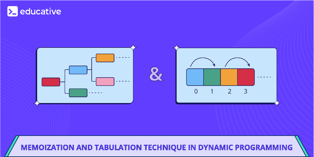
1. Memoization (Top-Down): This is the recursive approach. You start with the main problem and break it down. If you encounter a subproblem you've already solved, you use the stored answer. If not, you compute it, store it, and then use it.
2. Tabulation (Bottom-Up): This is the iterative approach we're focusing on today. You start with the smallest possible subproblems (the base cases) and solve them first. Then, you use these results to solve slightly larger subproblems, and so on, until you've built your way up to the solution for the original problem. You are essentially "filling a table" of results from the bottom up.

The Tabulation Process: A Fibonacci Example

Let's start with the familiar Fibonacci sequence.
Recurrence: $\text{Fib}(n)=\text{Fib}(n-1)+\text{Fib}(n-2)$
Base Cases: $\text{Fib}(0)=0,\text{Fib}(1)=1$

To solve this with tabulation, we follow a clear, mechanical process. The following video provides an excellent walkthrough of this exact process.

Let's summarize the four key steps of tabulation from the video:

1. Create the Table (DP Array): Create an array, often called dp, to store the solutions to subproblems. For Fib(n), we need an array of size n + 1 so that dp[i] can store the result of Fib(i).
2. Initialize Base Cases: Populate the array with the solutions to the smallest subproblems. Here, we'd set dp[0] = 0 and dp[1] = 1.
3. Iterate and Fill: Loop through the table, starting from the first unsolved subproblem, and apply the recurrence relation using the already-computed values in your table.

   # After initializing dp[0] and dp[1]
   for i in range(2, n + 1):
       dp[i] = dp[i-1] + dp[i-2]
   

4. Return the Answer: The final answer is the value in the table corresponding to the original problem, which is dp[n].

A Quick Note on Space Optimization

One of the benefits of the bottom-up approach is that it can make space optimizations more apparent. Notice that to calculate dp[i], we only need dp[i-1] and dp[i-2]. We don't need the entire array. This allows for a clever optimization.

While this is a powerful trick, your first goal should always be to get the standard tabulation solution working. Optimization comes second.

Tabulation in 1D: The Coin Change Problem

Let's apply this four-step process to a more complex problem you saw in the last lesson: Coin Change.

Problem: Given coins of different denominations and a total amount, find the fewest coins needed to make up that amount.

Recurrence: min_coins(m) = 1 + min(min_coins(m - c)) for every coin c where m >= c.
Base Case: min_coins(0) = 0.

Let's build the tabulation solution.

1. Create Table: We need to find the minimum coins for every amount from 0 to amount. So we create dp array of size amount + 1. dp[i] will store the minimum coins for amount i.
2. Initialize Base Cases: We know dp[0] = 0. For all other amounts, we don't yet know the answer. Since we're looking for a minimum, we should initialize them to a placeholder for infinity. In Python, float('inf') is perfect for this.
3. Iterate and Fill: We'll loop through each amount i from 1 to amount. For each amount, we'll try using each available coin.
   • If i - coin is a valid amount (i.e., >= 0), it means we can form amount i by taking one coin and adding it to the optimal solution for amount i - coin.
   • The number of coins in this case would be 1 + dp[i - coin].
   • We want the minimum over all possible coins, so we update dp[i] accordingly.
4. Return Answer: The final answer is dp[amount]. If it's still float('inf'), it means the amount was impossible to make.

The following resource provides a clean Python implementation of this logic.

Tabulation in 2D: The 0/1 Knapsack Problem

Some problems have a state that depends on more than one variable, leading to a 2D table (or a matrix). The 0/1 Knapsack Problem is a classic example.

Problem: Given a set of items, each with a weight and a value, determine the items to include in a collection so that the total weight is less than or equal to a given limit and the total value is as large as possible. You can either take an item or leave it (0/1).

State: The state needs to track two things: which items we are considering, and the current weight capacity of our knapsack. So, let dp[i][w] be the maximum value we can get using only the first i items with a maximum weight capacity of w.

Recurrence: For item i with value v_i and weight w_i:

• Option 1 (Don't take item i): The max value is the same as the max value using the first i-1 items with the same capacity w. This is dp[i-1][w].
• Option 2 (Take item i): We can only do this if w >= w_i. The value is v_i plus the max value we could get with the first i-1 items and the remaining capacity, w - w_i. This is v_i + dp[i-1][w - w_i].
  We take the maximum of these two options: dp[i][w] = max(dp[i-1][w], v_i + dp[i-1][w - w_i]).

Filling a 2D table can be tricky to visualize. The next resource provides an exceptionally detailed, cell-by-cell walkthrough. As the article suggests, grab a pen and paper and follow along!

Conclusion

You have now learned the essential mechanics of the bottom-up tabulation approach. This iterative method is a powerful and reliable way to implement any DP recurrence relation and is a cornerstone of competitive programming.

Key Takeaways:

• Tabulation is a bottom-up, iterative approach. You solve the smallest subproblems first and build up from there.
• The process is systematic:
  1. Create a table (1D, 2D, etc.) to store subproblem solutions.
  2. Initialize the base cases in the table.
  3. Use loops to iterate through the table, filling each entry using the recurrence relation and previously computed values.
  4. Return the final entry that corresponds to the solution of the original problem.
• Tabulation avoids recursion limits and can sometimes reveal space-saving optimizations.

Up Next:
In the next lesson, we will continue to practice our DP skills by applying them to another classic problem that uses a 2D table: the Longest Common Subsequence (LCS) problem. This will give you more experience with 2D DP and help you see the patterns that emerge across different problems.