Analyzing Space Complexity with Big-O Notation

1. What is Space Complexity?

Just as time complexity measures how runtime scales with input size, space complexity measures how memory usage scales. The Big-O notation you learned for time complexity applies in exactly the same way to space.

An algorithm uses memory for several things:

• Storing the program instructions themselves.
• Storing constant values and variables.
• Storing the input data.
• Storing any extra data structures it creates.
• Managing function calls (the call stack).

The following video provides a great introduction to the concept.

Total Space vs. Auxiliary Space

As the video explained, it's vital to distinguish between two types of space:

1. Input Space: The memory required to store the input data provided to the algorithm. For a list of n integers, this is O(n).
2. Auxiliary Space: The extra or temporary memory that an algorithm requires to run, excluding the input space.

When we analyze space complexity in competitive programming, we are most often concerned with the auxiliary space. The problem statement defines the input size, and we can't change that. What we can control is how much extra memory our algorithm allocates. An algorithm that uses O(1) auxiliary space is called an in-place algorithm.

For example, if a function takes a list of size n and sorts it without creating any new lists, its input space is O(n) but its auxiliary space is O(1). If it creates a new, sorted copy of the list, its auxiliary space is O(n).

2. Common Space Complexities

Let's explore the most common space complexities with Python examples.

O(1) — Constant Space

An algorithm has constant space complexity if its memory usage does not depend on the input size. It uses a small, fixed amount of memory for variables, regardless of how large n is.

# This function uses O(1) auxiliary space.
# The memory for 'total' and 'i' does not change with the size of the list.
# The input 'numbers' itself takes O(n) space, but that's input space.
def sum_list_in_place(numbers):
    total = 0  # One variable
    for num in numbers:
        total += num
    return total

This is an in-place operation. Another example is modifying an input directly, which avoids allocating new memory.

The next resource demonstrates the contrast between an algorithm that creates a new data structure and one that modifies the input in-place.

O(n) — Linear Space

An algorithm has linear space complexity if its memory usage grows in direct proportion to the input size n. This typically happens when you create a data structure that contains n elements.

# This function uses O(n) auxiliary space
# because it creates a new list 'squared_numbers' of size n.
def square_all_numbers(numbers):
    n = len(numbers)
    squared_numbers = [0] * n  # A new list of size n is created
    for i in range(n):
        squared_numbers[i] = numbers[i] ** 2
    return squared_numbers

Another common O(n) pattern in competitive programming is using a hash map (dictionary in Python) or a set to keep track of seen elements from an input of size n.

def find_unique_elements(items):
    seen = set()
    for item in items:
        seen.add(item)
    
    unique_list = list(seen)
    return unique_list

Other Complexities

While O(1) and O(n) are the most common, you'll also encounter others:

• O(log n) — Logarithmic Space: This is rare but very efficient. It often occurs in recursive algorithms where the number of recursive calls on the stack at any one time is proportional to log n. Recursive binary search is a classic example.
• O(n²) — Quadratic Space: Memory usage grows with the square of the input size. This is common when creating a 2D grid or an adjacency matrix for a graph with n vertices, which requires n x n space.

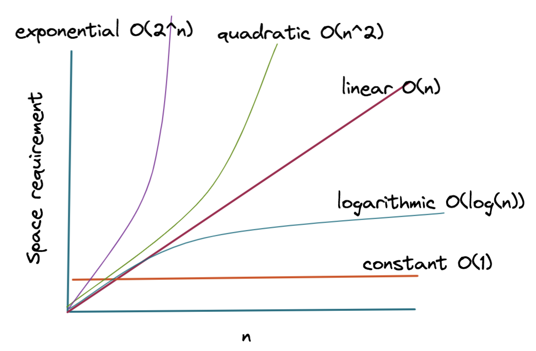
This graph, which we saw in the last lesson, applies equally well to space complexity. It shows how quickly O(n^2) can become impractical compared to O(n) or O(1).

3. The Special Case: Recursion and the Call Stack

Recursion is a powerful technique, but it has a hidden cost: space. Every time a function calls itself, the system must save its current state (local variables, parameters, return address) on the call stack. Each of these saved states is called a stack frame.

The space complexity of a recursive algorithm is determined by the maximum depth of the call stack.

The next video does an exceptional job of comparing an iterative and a recursive solution for the same problem (factorial), highlighting how the call stack impacts space complexity.

As you saw, the key takeaway is:

• Iterative Factorial: Uses O(1) auxiliary space. A few variables are used, and their memory doesn't grow with n.
• Recursive Factorial: Uses O(n) auxiliary space. For an input n, the call stack grows to a depth of n, with each call adding a new frame to the stack.

This is why a naive recursive solution can easily cause a "Memory Limit Exceeded" or "Stack Overflow" error for large n in a programming contest.

4. Practical Analysis and Trade-offs

When choosing an algorithm, you often face a time-space trade-off. Sometimes, you can achieve a faster runtime by using more memory, or save memory at the cost of a slower runtime.

• Memoization (a technique we'll study in detail later) is a classic example. We store the results of expensive function calls in a dictionary (O(n) space) to avoid re-computing them, drastically improving time complexity.

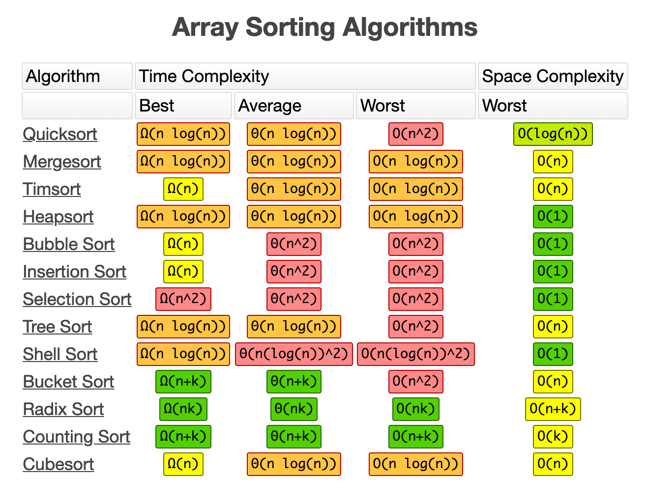
The table below shows the space complexity for common sorting algorithms. Notice how some, like Heap Sort, are in-place (O(1) space), while others, like Merge Sort, require extra memory (O(n) space). This is a practical trade-off you might make depending on the problem's constraints.

To analyze a new algorithm's space complexity, you can follow these steps, adapted from the article "Space Complexity: How Algorithms Use Memory" by DataCamp:

1. Clarify scope: Are you calculating auxiliary space or total space? (For CP, it's usually auxiliary).
2. Count fixed-size variables: These contribute O(1).
3. Measure auxiliary data structures: Measure arrays, lists, sets, and dictionaries relative to the input size (n). A list of n items is O(n). A 2D array of n x n is O(n²).
4. Calculate recursion depth: For recursive algorithms, the maximum depth of the call stack determines its space contribution.
5. Combine and simplify: Sum the space from all components and express the result using the tightest Big-O bound.

Conclusion

You now have the tools to analyze both the time and space efficiency of your code—the two pillars of performance in competitive programming.

Key Takeaways:

• Space Complexity measures how an algorithm's memory usage scales with input size, using Big-O notation.
• Auxiliary Space is the extra memory an algorithm allocates, excluding the input. This is the primary focus for optimization in competitive programming.
• Common space complexities are O(1) (constant/in-place), O(n) (linear), and O(n²) (quadratic).
• Recursion consumes space via the call stack. The space complexity is proportional to the maximum recursion depth.
• Often, there is a time-space trade-off, where you can use more memory to make an algorithm faster.

Up Next:

In the next lessons, we'll solidify these analysis skills by learning to quickly recognize common complexity patterns in code. We'll start by taking a closer look at how to identify common time complexities (logarithmic, linear, quadratic) from code patterns, which will make you faster and more accurate in your initial assessment of a problem.