Level Order Traversal with Queues

1. Breadth-First vs. Depth-First Traversal

The name "level-order traversal" perfectly describes the process. We visit all nodes on level 0 (the root), then all nodes on level 1, then all on level 2, and so on. This "wide before deep" approach is the essence of Breadth-First Search.

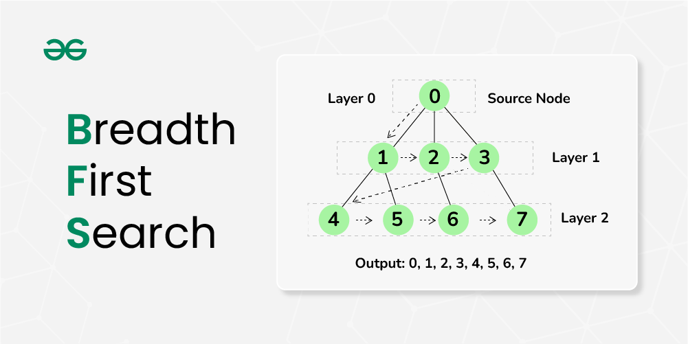
The key to achieving this lies in the data structure we use. While iterative DFS relied on a stack (Last-In, First-Out), BFS relies on a queue (First-In, First-Out).

Think of it like waiting in a line: the first person to get in line is the first person to be served. In our traversal, the first node we add to our "to-visit" list (the root) is the first one we process. This simple FIFO principle ensures we exhaust an entire level before moving to the next.

2. The BFS Algorithm with a Queue

The algorithm for level-order traversal is intuitive and elegant. It follows these steps:

1. Create a queue and add the root node to it.
2. Start a loop that continues as long as the queue is not empty.
3. Inside the loop, dequeue a node (remove it from the front of the queue).
4. "Visit" the dequeued node (e.g., add its value to a results list).
5. Enqueue the node's left child, if it exists (add it to the back of the queue).
6. Enqueue the node's right child, if it exists (add it to the back of the queue).

To see this process in action, watch the following conceptual overview.

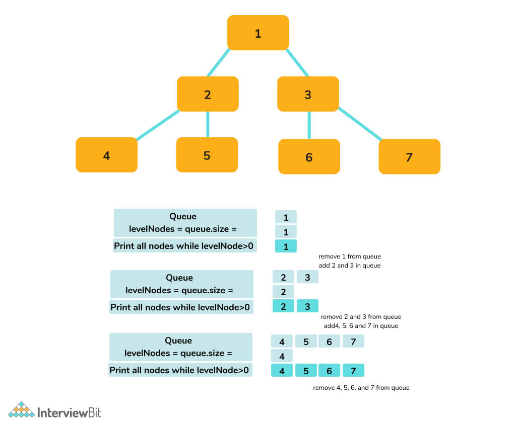
The following diagram provides another static, step-by-step view of the process, reinforcing what you saw in the video.

3. Implementation: Grouping Nodes by Level

A common requirement in competitive programming problems, like LeetCode's "Binary Tree Level Order Traversal", is to return the result as a list of lists, where each inner list contains the nodes of a single level.

Our basic BFS algorithm gives us a single flat list. How can we modify it to group the nodes? The solution is a clever but simple extension.

Before processing a level, we can check the current size of the queue. That size tells us exactly how many nodes are on the current level. We can then run an inner loop that many times to process only the nodes of that level.

The following resource explains this crucial pattern in detail.

Let's look at the complete Python code. We'll use collections.deque, which is a highly efficient implementation of a queue in Python, providing $O(1)$ time complexity for append (enqueue) and popleft (dequeue) operations.

from collections import deque

# Assume this TreeNode class is defined from previous lessons
class TreeNode:
    def __init__(self, val=0, left=None, right=None):
        self.val = val
        self.left = left
        self.right = right

def level_order_traversal(root: TreeNode):
    # Handle the edge case of an empty tree
    if not root:
        return []

    result = []
    queue = deque([root])  # Initialize the queue with the root node

    while queue:
        # 1. Get the number of nodes at the current level
        level_size = len(queue)
        current_level_nodes = []

        # 2. Loop exactly that many times to process all nodes at this level
        for _ in range(level_size):
            # 3. Dequeue a node from the front
            node = queue.popleft()
            current_level_nodes.append(node.val)

            # 4. Enqueue its children for the next level
            if node.left:
                queue.append(node.left)
            if node.right:
                queue.append(node.right)
        
        # 5. Add the completed level to the result
        result.append(current_level_nodes)

    return result

To solidify your understanding, watch this part of the NeetCode video where the instructor implements this exact logic.

      10
     /  \
    5    15
   / \    \
  3   7    18

4. Complexity Analysis

Understanding the performance of this algorithm is crucial for competitive programming.

• Time Complexity: $O(N)$
  We visit every node in the tree exactly once. Each node is enqueued and dequeued once. Therefore, the time complexity is linear with respect to the number of nodes, $N$.

• Space Complexity: $O(W)$ or $O(N)$
  The space complexity is determined by the maximum number of nodes stored in the queue at any given time. This corresponds to the maximum width ($W$) of the tree. In the worst-case scenario for a binary tree (a complete or "bushy" tree), the last level can contain up to $(N+1)/2$ nodes. Therefore, the worst-case space complexity is $O(N)$.

Conclusion

You have now mastered a second major tree traversal strategy: level-order traversal (or BFS). By understanding the roles of both stacks (for DFS) and queues (for BFS), you have significantly expanded your algorithmic toolkit.

Key Takeaways:

• Level-order traversal explores a tree layer by layer, which is a form of Breadth-First Search (BFS).
• The core data structure for BFS is a queue (First-In, First-Out), efficiently implemented in Python with collections.deque.
• To group nodes by level, a common pattern is to use a nested loop: an outer while loop to continue traversal and an inner for loop that iterates len(queue) times to process a single level.
• The algorithm has a time complexity of $O(N)$ and a worst-case space complexity of $O(N)$.

Up Next:
With a solid grasp of both depth-first and breadth-first traversals, you are now equipped to tackle a wide variety of tree-based problems. In our next lesson, we will apply these traversal techniques to solve problems involving tree properties, such as calculating a tree's height or finding its diameter. You'll see how choosing the right traversal strategy can make solving these problems much more straightforward.