Dot Products: Calculation and Geometry

Welcome to the second lesson in our series on the mathematical foundations of machine learning. In our last session, we refreshed our understanding of vectors and the basic operations of addition, scaling, and measuring their length (norm). Now, we'll build on that foundation to explore one of the most important operations in all of linear algebra: the dot product.

This lesson will show you how to "multiply" two vectors to get a single number—a scalar—and, more importantly, what that number tells you about the vectors' geometric relationship. Understanding the dot product is crucial, as it forms the basis for measuring vector similarity, determining orthogonality, and is a core computational step in many machine learning algorithms, including neural networks.

1. Computing the Dot Product: The Algorithmic View

Let's start with the mechanics. The dot product of two vectors is found by multiplying their corresponding components and then summing the results.

For two vectors $a$ and $b$ of the same dimension $n$ , their dot product (also called the inner product) is defined as:

a \cdot b = a_{1} b_{1} + a_{2} b_{2} + \dots + a_{n} b_{n} = i = 1 \sum n a_{i} b_{i}

The result is always a single number (a scalar), not a vector.

For example, let's take two vectors in $R^{3}$ :

a = 2 - 1 3, b = 45 - 2

Their dot product is:

a \cdot b = (2) (4) + (- 1) (5) + (3) (- 2) = 8 - 5 - 6 = - 3

This "piece-by-piece" multiplication is visualized well in the following image for a 2D case.

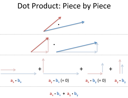
This diagram illustrates the component-wise multiplication that forms the dot product. The x-components are multiplied together, and the y-components are multiplied together, before being summed.

There are several common notations for the dot product that you'll see in ML literature:

$a \cdot b$ (dot notation)
$a^{T} b$ (matrix multiplication notation, which will make more sense in our next lesson)
$⟨ a, b ⟩$ (inner product notation)

To see this in a practical context, let's watch a short video that covers the calculation and its implementation in common Python libraries.

The Dot Product — Topic 14 of Machine Learning Foundations

Watch these clips from "The Dot Product" by Jon Krohn.

Start with the introduction to notations. Next, watch the clear explanation of the calculation process. Finally, see how it's done in code by watching the NumPy implementation. The PyTorch and TensorFlow sections are also interesting but the NumPy example is sufficient to see the principle in action.

2. The Geometric Interpretation: What the Dot Product Means

The real power of the dot product comes from its geometric meaning. It tells us about the alignment of two vectors. There are two deeply connected ways to think about this.

Interpretation 1: Projection

The dot product relates to projecting one vector onto another.

The dot product $v \cdot w$ is the length of the projection of $w$ onto $v$ , multiplied by the length of $v$ .

Let's watch a segment from 3Blue1Brown that provides a fantastic visual intuition for this idea.

Dot products and duality | Chapter 9, Essence of linear algebra

Watch "Dot products and duality" from the Essence of linear algebra series.

First, focus on the core geometric intuition involving projection. Pay close attention to how the sign of the dot product changes depending on whether the vectors point in similar or opposite directions. Then, watch the explanation for why order doesn't matter (\vec{v} \cdot \vec{w} = \vec{w} \cdot \vec{v}). This is a key property called commutativity.

As the video explained, the sign of the dot product gives us a quick way to gauge the angle between two vectors:

$a \cdot b > 0$ : The vectors are pointing in generally the same direction. The angle $θ$ between them is less than 90° ( $θ < 9 0^{\circ}$ ).
$a \cdot b = 0$ : The vectors are perpendicular, or orthogonal. The angle between them is exactly 90° ( $θ = 9 0^{\circ}$ ). This is a critical test for orthogonality.
$a \cdot b < 0$ : The vectors are pointing in generally opposite directions. The angle $θ$ between them is greater than 90° ( $θ > 9 0^{\circ}$ ).

Interpretation 2: The Cosine Formula

The projection-based view leads directly to a very useful formula involving the angle, $θ$ , between the two vectors.

This diagram shows the relationship between vectors $\vec{a}$ and $\vec{b}$, the angle $\theta$ between them, and the component of $\vec{a}$ projected onto $\vec{b}$, which is $\lVert\vec{a}\rVert \cos(\theta)$.

The length of the projection of $a$ onto $b$ is $∥ a ∥ cos (θ)$ . Based on our first interpretation (projecting $a$ onto $b$ and multiplying by the length of $b$ ), we get the cosine formula for the dot product:

a \cdot b = ∥ a ∥ ∥ b ∥ cos (θ)

Here, $∥ a ∥$ and $∥ b ∥$ are the L2 norms (lengths) of the vectors, which we covered in the previous lesson. This formula elegantly bridges the gap between the component-wise algebraic calculation and the geometry of angles and lengths.

The following reading explains this connection very clearly.

Linear Algebra 101 for AI/ML – Part 2 - Backprop

This article from Backprop provides an excellent visual breakdown of the geometric perspective.

Start at the section "Visual Perspective" and read down to the end of the three cases (a \cdot b > 0, a \cdot b < 0, a \cdot b = 0). Focus on how the cosine formula is derived from the idea of projection. The diagrams are particularly helpful for visualizing this.

A powerful application of this formula is that it allows us to calculate the angle between any two vectors, provided we know their components:

cos (θ) = \frac{a \cdot b}{∥ a ∥ ∥ b ∥}

This equation is fundamental in machine learning for measuring the similarity between vectors, often called cosine similarity. If two vectors point in the exact same direction, $θ = 0^{\circ}$ , $cos (θ) = 1$ , and the similarity is maximal. If they are orthogonal, $θ = 9 0^{\circ}$ , $cos (θ) = 0$ , and they have no similarity.

3. Practice Problems

Let's test your understanding. Given the vectors:

v = [34], w = [- 8 6]

Calculate the dot product $v \cdot w$ .
Based on the sign of the dot product, what can you conclude about the angle between $v$ and $w$ ?
Calculate the angle $θ$ between $v$ and $w$ in degrees.

Take a few minutes to work through these before checking the solutions.

Solutions

Dot Product Calculation:
$v \cdot w = (3) (- 8) + (4) (6) = - 24 + 24 = 0$
Conclusion from the Sign:
Since the dot product is 0, the vectors $v$ and $w$ are orthogonal (perpendicular).
Angle Calculation:
First, we need the norms of the vectors.
$∥ v ∥ = 3^{2} + 4^{2} = 9 + 16 = 25 = 5$ $∥ w ∥ = (- 8)^{2} + 6^{2} = 64 + 36 = 100 = 10$
Now, use the cosine formula:
$cos (θ) = \frac{v \cdot w}{∥ v ∥ ∥ w ∥} = \frac{0}{( 5 ) ( 10 )} = 0$
The angle $θ$ for which $cos (θ) = 0$ is $9 0^{\circ}$ .
$θ = arccos (0) = 9 0^{\circ}$

Conclusion

In this lesson, we explored the dot product from both a computational and a geometric perspective. It's a simple operation with profound implications.

Key Takeaways:

The dot product is computed by taking the sum of the element-wise products of two vectors, resulting in a scalar.
Geometrically, the dot product is the length of one vector multiplied by the length of the second vector's projection onto the first.
The sign of the dot product indicates alignment: positive for similar directions, negative for opposing directions, and zero for orthogonal vectors.
The cosine formula, $a \cdot b = ∥ a ∥ ∥ b ∥ cos (θ)$ , connects the algebraic and geometric views and is used to find the angle between vectors.

The dot product is not just an abstract tool; it's used everywhere in ML, from calculating the output of a single neuron to measuring the similarity of documents for a search engine.

In our next lesson, we will expand our scope from vectors to matrices and explore matrix multiplication, an operation that is built upon the foundation of the dot product. You'll see how the $a^{T} b$ notation fits into this larger picture.