KL Divergence in Variational Inference: Mode-Seeking vs. Mode-Covering

1. Forward vs. Reverse KL: A Formal Distinction

Let's establish our notation. We have a true, complex data distribution $P$ that we want to approximate with a simpler model distribution $Q$. The two ways we can measure the divergence are:

1. Forward KL Divergence: $D_{KL}(P\Vert Q)$

   $$D_{KL}(P\Vert Q)=\sum _{x}P(x)\log \frac{P(x)}{Q(x)}={\mathbb{E}}_{x\sim P}\left[\log \frac{P(x)}{Q(x)}\right]$$

   This is used in scenarios like standard maximum likelihood estimation. Minimizing this is equivalent to minimizing the cross-entropy $H(P,Q)$, as $H(P)$ is constant with respect to $Q$.

2. Reverse KL Divergence: $D_{KL}(Q\Vert P)$

   $$D_{KL}(Q\Vert P)=\sum _{x}Q(x)\log \frac{Q(x)}{P(x)}={\mathbb{E}}_{x\sim Q}\left[\log \frac{Q(x)}{P(x)}\right]$$

   As we saw, variational inference minimizes a form of this: $D_{KL}(q_{\varphi }(z|x)\Vert p_{\theta }(z|x))$, where $Q$ is our tractable approximation $q$ and $P$ is the intractable target $p$.

The crucial difference lies in the expectation. Forward KL is an expectation over the true distribution $P$, while Reverse KL is an expectation over the approximation $Q$. This seemingly small change leads to vastly different optimization landscapes and behaviors.

2. The Penalty Game: Mode-Covering vs. Mode-Seeking

The core intuition for why these two objectives behave differently comes from analyzing their behavior when probabilities are near zero. This is where the logarithm term can dominate.

Let's think about what each objective penalizes most harshly:

• Forward KL ($D_{KL}(P\Vert Q)$): Consider a point $x$ where the true probability $P(x)$ is high, but our approximation $Q(x)$ is near zero. The term $\log \frac{P(x)}{Q(x)}$ will become very large, and since it's weighted by $P(x)$, the overall divergence will explode. To avoid this infinite penalty, the approximation $Q$ is forced to have non-zero mass wherever $P$ has mass. It must "cover" the entire support of $P$. If $P$ is multimodal, $Q$ will tend to spread itself out to cover all the modes, often resulting in a single, broad distribution that averages them. This is known as mode-covering or mean-seeking behavior.

• Reverse KL ($D_{KL}(Q\Vert P)$): Now consider a point $x$ where our approximation $Q(x)$ is high, but the true probability $P(x)$ is near zero. The term $\log \frac{Q(x)}{P(x)}$ will again become very large, and since it's weighted by $Q(x)$, the divergence explodes. To avoid this, the approximation $Q$ is forced to be zero (or very small) wherever $P$ is zero. It is penalized for placing probability mass in regions that are impossible under the true distribution. This is a "zero-forcing" property. Conversely, if $P(x)$ is high but $Q(x)$ is zero, the contribution to the sum is zero. This means $Q$ is not penalized for missing a mode of $P$. It is free to pick one mode of $P$ and focus all its mass there, ensuring it doesn't place mass in the low-probability regions between modes. This is known as mode-seeking behavior.

The following article provides an excellent, detailed explanation of this phenomenon, complete with interactive visualizations.

The video below also offers a concise and intuitive animated explanation of this core difference.

3. A Clearer Picture

The image below provides a static but powerful visualization of this exact scenario. Here, the true distribution $p$ is a mixture of two Gaussians. We are trying to fit it with a single Gaussian, $q$. The plots show the value of the KL divergence for different parameters (mean $\mu$ and standard deviation $\sigma$) of our approximation $q$. The darker regions represent lower KL divergence, which is our goal.

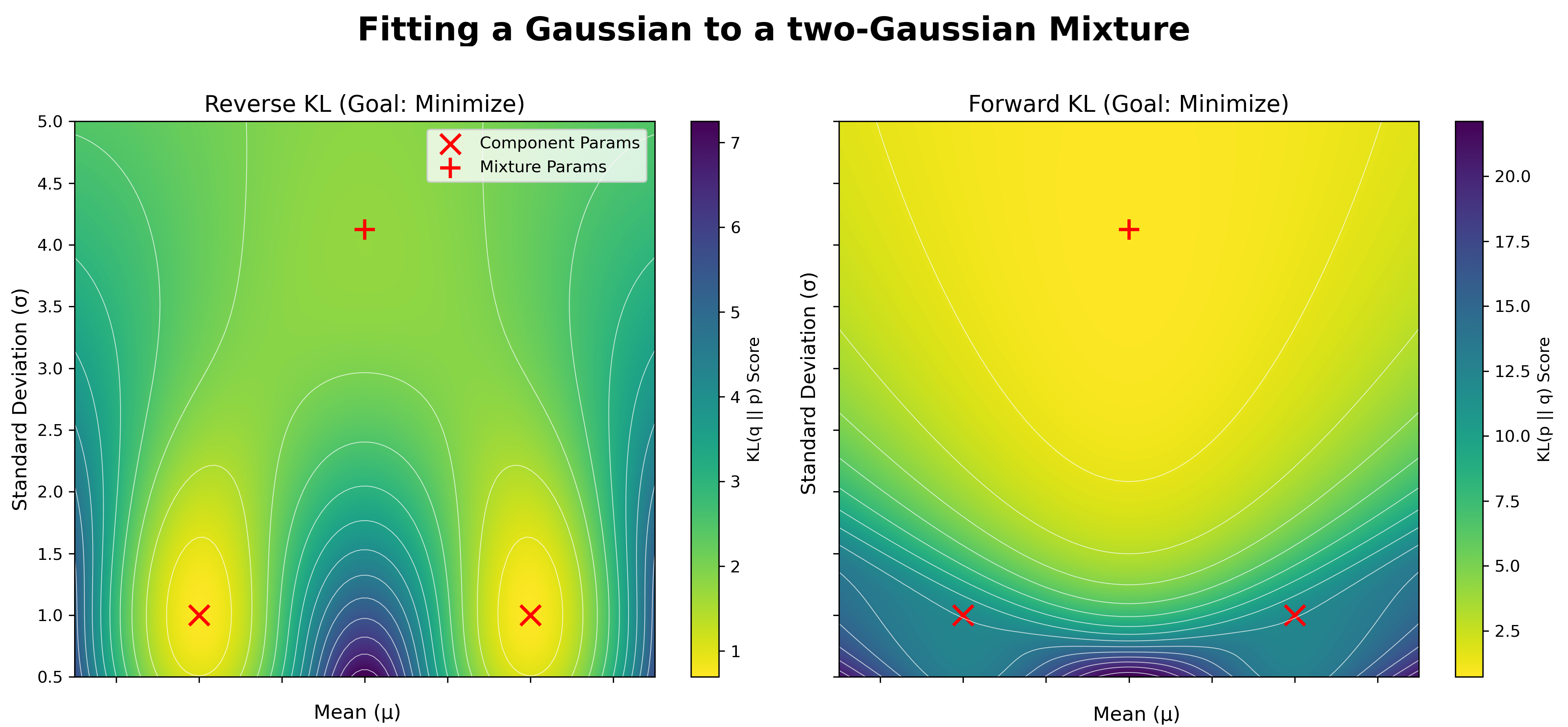
Let's analyze the two plots:

• Reverse KL (Left Plot): This shows the landscape for minimizing $D_{KL}(q\Vert p)$, the objective used in variational inference. Notice that there are two distinct minima. The optimal strategy for $q$ is to place its mass squarely over one of the two modes of $p$. It "seeks" a single mode and ignores the other. This is a classic mode-seeking landscape.

• Forward KL (Right Plot): This shows the landscape for minimizing $D_{KL}(p\Vert q)$. Here, there is only one broad, shallow minimum located between the two modes of $p$. The optimal $q$ becomes wide and averages the two modes, trying to "cover" the entire region where $p$ has mass. This is a classic mode-covering landscape.

4. Why Variational Inference Uses Reverse KL

Now we can answer the crucial question: why do VAEs and other variational methods minimize the reverse KL, $D_{KL}(q\Vert p)$? There are two main reasons.

1. Practicality and Tractability:
This is the most compelling reason. The Reverse KL objective is ${\mathbb{E}}_{z\sim q}[\log (q(z)/p(z))]$. The expectation is taken with respect to our simple, approximate distribution $q$. This means we can estimate the objective by drawing samples from $q$—something we can easily do by design—and evaluating the term inside the expectation. This is the foundation of the reparameterization trick and Monte Carlo estimation of the ELBO.

If we were to use Forward KL, the objective would be ${\mathbb{E}}_{z\sim p}[\log (p(z)/q(z))]$. The expectation is with respect to the true posterior $p$. But $p$ is precisely the intractable distribution we're trying to avoid! We cannot sample from it, so we cannot compute this objective. The choice of Reverse KL is, therefore, a deeply pragmatic one that makes the entire variational inference framework computationally feasible.

The video below, which you may recall from the previous lesson, frames the optimization problem in exactly this way, setting up the minimization of $D_{KL}(Q\Vert P)$ because it's the only tractable path forward.

2. Desirability of Mode-Seeking:
While the practical reason is paramount, the behavioral consequence is also often desirable. In many inference tasks, we want our model to produce a confident, unambiguous explanation. The mode-seeking nature of Reverse KL encourages the approximate posterior to find a single, high-density region in the latent space that corresponds to the input data. While this might lead to ignoring other, less likely interpretations (modes), it often results in sharper and more useful representations for tasks like generation.

Conclusion

In this lesson, we've unpacked the crucial asymmetry of KL divergence and understood its profound impact on optimization.

Key Takeaways:

• Forward KL ($D_{KL}(P\Vert Q)$) is mode-covering. It penalizes the model $Q$ for missing regions where the true distribution $P$ has mass, forcing $Q$ to spread out and average over the modes of $P$.
• Reverse KL ($D_{KL}(Q\Vert P)$) is mode-seeking. It penalizes the model $Q$ for assigning probability where $P$ has none, forcing $Q$ to be selective and focus on a single mode of $P$.
• Variational Inference uses Reverse KL for two primary reasons:
  1. Tractability: The objective's expectation is with respect to the simple distribution $Q$, making it computable via sampling.
  2. Behavior: The resulting mode-seeking property often leads to sharp, confident latent representations.

This lesson concludes our module on Estimation and Inference. You now have a comprehensive understanding of the theory behind VAEs, from the individual information-theoretic building blocks to the full ELBO objective and the nuances of its optimization.

In our next module, we will pivot to a new area: Stochastic Processes. We'll start by revisiting the concept of Markov chains and exploring their properties, which form the essential mathematical groundwork for understanding the forward and reverse processes in Denoising Diffusion Probabilistic Models (DDPMs), the final paper you aim to implement.