Convexity in Optimization

1. Defining Convexity

The term "convex" has a very specific mathematical meaning, but it aligns well with our intuition of a "bowl-shaped" object or function. We can define convexity for sets, functions, and entire optimization problems.

Let's begin with a visual introduction to these ideas. The following short video provides clear, intuitive definitions for convex sets and functions.

As the video illustrates, the core ideas are:

• Convex Set: A set $S$ is convex if for any two points $x_0,x_1\in S$, the entire line segment connecting them also lies within $S$. Mathematically, $(1-\lambda )x_0+\lambda x_1\in S$ for all $\lambda \in [0,1]$.
• Convex Function: A function $f$ is convex if its epigraph—the set of all points lying on or above its graph—is a convex set. This is what gives rise to the characteristic "bowl shape."

The formal definition of a convex function, also known as Jensen's inequality, states that the function's value at a convex combination of two points is less than or equal to the convex combination of the function's values at those points.

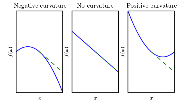
Geometrically, this means the chord connecting any two points on the function's graph lies on or above the graph itself.

2. The Hessian Test for Convexity

While the geometric and algebraic definitions are fundamental, they can be difficult to apply directly to a function given by a formula. For twice-differentiable functions, there is a much more direct and powerful test that uses the Hessian matrix, which we introduced in the last lesson.

The key result is:
A smooth (twice-differentiable) function is convex if and only if its Hessian matrix is positive semidefinite everywhere in its domain.

Let's break this down.

• A matrix $\mathbf{H}$ is positive semidefinite (PSD) if for any non-zero vector $\mathbf{v}$, the quadratic form ${\mathbf{v}}^T\mathbf{Hv}\ge 0$. This means the function has non-negative curvature in all directions.
• A symmetric matrix (like the Hessian) is positive semidefinite if and only if all of its eigenvalues are non-negative (${\lambda }_i\ge 0$).

This gives us a practical algorithm for checking convexity: compute the Hessian matrix, find its eigenvalues, and check if they are all greater than or equal to zero for all points in the function's domain.

The following reading from a University of Toronto lecture formalizes this connection.

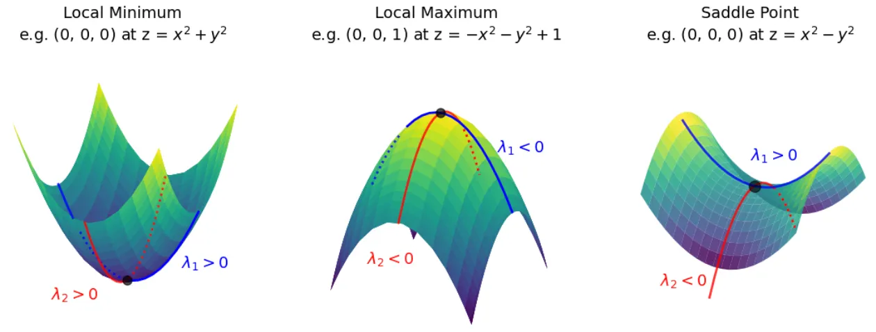
At a local minimum, the Hessian must be at least positive semidefinite. If it's strictly positive definite (all eigenvalues > 0), the function curves upwards in every direction, forming a distinct "bowl." If the Hessian is indefinite (some positive, some negative eigenvalues), we are at a saddle point, which curves up in some directions and down in others.

3. Why Convexity is the Holy Grail of Optimization

Now that we have a tool to identify convex functions, let's explore why this property is so desirable. The main reason is that for convex functions, any local minimum is also a global minimum.

This property dramatically simplifies optimization. It means we don't have to worry about getting stuck in "spurious" local minima that are not the best overall solution. If we find a point where the gradient is zero, and we know the function is convex, we have found the global minimum.

The video we watched earlier provides a beautiful explanation for this property.

This is a powerful result. For a convex function $f$, the first-order Taylor approximation provides a global lower bound:

If we find a point $x^{\ast }$ where $\nabla f(x^{\ast })=0$, the inequality simplifies to $f(x)\ge f(x^{\ast })$ for all $x$. This proves that $x^{\ast }$ is a global minimum.

4. Convexity in Deep Learning

Given the wonderful properties of convex optimization problems, it's natural to ask: is training a neural network a convex problem?

The answer is a definitive no.

The loss landscapes of deep neural networks are highly non-convex. A simple and elegant argument for this involves the symmetry of hidden units.

The argument, as you just read, is that you can swap the hidden units in a layer (and their corresponding weights) without changing the function computed by the network. This creates multiple, distinct parameter vectors that yield the exact same loss value. If the loss function were convex, the average of these parameter vectors would have to give a loss less than or equal to the original loss. However, averaging the weights of permuted units typically leads to a degenerate, poorly performing network. This contradiction proves the loss landscape cannot be convex.

This inherent non-convexity is the primary reason optimization in deep learning is so challenging and is an active area of research. It's why we have to contend with complex landscapes filled with saddle points, plateaus, and multiple local minima, and why we need sophisticated optimizers like Adam, which we will analyze later in this module.

Conclusion

In this lesson, we established a formal understanding of convexity, a cornerstone of optimization theory.

Key Takeaways:

• Convex sets contain the line segment between any two of their points.
• Convex functions are "bowl-shaped," meaning the chord between any two points on their graph lies above the function.
• The crucial Hessian test states that a twice-differentiable function is convex if and only if its Hessian matrix is positive semidefinite (PSD) everywhere. This is equivalent to all eigenvalues of the Hessian being non-negative.
• The power of convexity lies in the fact that for a convex function, any local minimum is also a global minimum, which greatly simplifies optimization.
• Training a deep neural network is a non-convex optimization problem, primarily due to symmetries in the network architecture.

You now have the tools to identify a convex problem and understand why it is fundamentally more tractable than a non-convex one.

In our next lesson, we will begin our study of the algorithms designed to navigate these landscapes. We will derive the gradient descent update rule from first principles and analyze its convergence properties, starting with the idealized case of smooth convex functions.