Learning Rate Schedules and Training Dynamics

1. The Rationale for Learning Rate Schedules

Why not just pick one good learning rate and stick with it? The answer lies in the changing nature of the optimization process. The training dynamics at the beginning, middle, and end of a run call for different step sizes.

• Early Training (Exploration): The model starts from a random initialization, far from any optimal solution. Here, we want to make rapid progress, which suggests a larger learning rate. However, the loss landscape can be highly curved or "sharp," and a large learning rate can cause the optimizer to take unstable steps, leading to divergence.
• Mid-Training (Convergence): As the model finds a promising broad basin in the loss landscape, the gradients become more consistent. We need to decrease the learning rate to begin converging towards the minimum within that basin.
• Late Training (Refinement): Near a local minimum, the gradients are small and noisy. To settle precisely into the minimum without oscillating around it, we need a very small learning rate.

This tradeoff between rapid initial progress and stable final convergence is the fundamental reason we use learning rate schedules. A good schedule manages the learning rate to suit each phase of training. The following article provides an excellent deep dive into this topic.

2. Stabilizing the Start: Learning Rate Warmup

As discussed, starting with a high learning rate can be catastrophic. The optimizer, faced with large gradients from a random initialization, can "explode" the loss. To prevent this, we introduce a warmup phase.

The idea is simple: begin with a very small learning rate and gradually increase it to a target maximum value over a set number of initial steps. This allows the optimizer to "get its bearings" and find a stable direction before we start taking larger, more exploratory steps. Warmup is especially critical when using adaptive optimizers like Adam, as it helps stabilize the initial, noisy moment estimates.

The following resource provides a more formal, theoretical perspective on why warmup is so effective, connecting it to the local curvature of the loss function—a concept that may resonate with your mathematical background.

3. The Modern Standard: Warmup and Cosine Decay

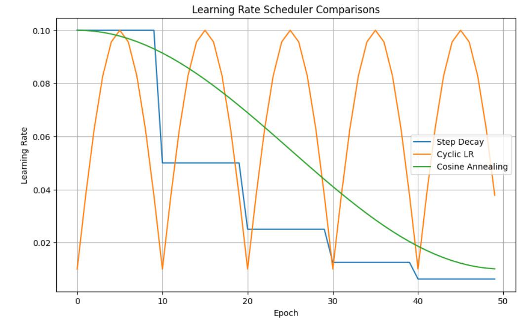
Once the warmup phase is complete, we need to begin decaying the learning rate. While simple schedules like step decay (reducing the LR at fixed intervals) or linear decay exist, the most effective and widely adopted method today is cosine decay.

Instead of dropping the learning rate in jarring steps, the cosine schedule smoothly decreases it from its maximum value ${\eta }_{\max }$ down to a minimum value ${\eta }_{\min }$ following the shape of a half-cosine wave.

The formula for cosine decay over $T$ total steps is:

Let's break this down:

1. As the current step $t$ goes from 0 to $T$, the term $\frac{\pi t}{T}$ goes from 0 to $\pi$.
2. $\cos \left(\frac{\pi t}{T}\right)$ therefore traces the cosine curve from $\cos (0)=1$ to $\cos (\pi )=-1$.
3. The term $\frac{1}{2}(1+\cos (\dots ))$ shifts and scales this to the range $[1,0]$. This is often called the "raised cosine".
4. This [1, 0] multiplier is then used to interpolate linearly between ${\eta }_{\max }$ and ${\eta }_{\min }$.

The shape of this decay is what makes it so effective. The learning rate decreases slowly at the beginning, allowing for continued exploration after the warmup. The decay then accelerates through the middle of training, corresponding to the phase where the model is rapidly converging. Finally, the decay slows down again as it approaches ${\eta }_{\min }$, allowing for fine-grained refinement.

To see this more clearly, let's examine the derivative of $\eta (t)$ with respect to $t$:

The rate of decay is proportional to $\sin (\pi t/T)$. This means the decay is slowest at the start ($t=0$) and end ($t=T$), and fastest exactly in the middle of training ($t=T/2$), perfectly matching the desired training dynamics.

The combination of a linear warmup followed by a cosine decay is the de facto standard for training large models like Transformers.

4. An Extension: Cosine Annealing with Warm Restarts

A powerful variant of cosine decay is Stochastic Gradient Descent with Warm Restarts (SGDR). Instead of one long decay over the entire training run, the learning rate is periodically "restarted" by resetting it to ${\eta }_{\max }$ and beginning a new, often shorter, cosine decay cycle.

Why would we do this? A key motivation is to escape sharp local minima. As the learning rate anneals to a small value, the optimizer might settle into a narrow, sharp valley in the loss landscape. Such minima often correspond to models that generalize poorly. A sudden increase in the learning rate provides a "kick" that can propel the optimizer out of this sharp minimum, allowing it to continue exploring for wider, flatter minima that lead to better generalization.

The following video from Stanford's CS231n course gives a good high-level overview of various scheduling strategies, including cosine decay and warmup.

For a deeper look into warm restarts, the article we've been using is once again an excellent resource.

Conclusion

In this lesson, we've moved beyond a static learning rate and explored the dynamics of scheduling. We saw that controlling the global learning rate over time is critical for balancing the need for fast exploration with stable convergence.

Key Takeaways:

• Learning rate schedules adapt the learning rate to the different phases of optimization, improving both training speed and final model performance.
• Warmup is a crucial initial phase where the learning rate is gradually increased to prevent instability when starting with random weights.
• Cosine decay provides a smooth, theoretically-motivated schedule that decreases the learning rate slowly at the start and end of training, and more rapidly in the middle.
• The combination of linear warmup and cosine decay is the state-of-the-art recipe for training large-scale deep learning models, including the Transformers you'll be implementing.
• Warm restarts can further improve generalization by periodically resetting the learning rate, helping the optimizer escape sharp minima.

We have now covered the core components of modern optimizers and their scheduling. However, the loss landscapes of deep networks present challenges beyond ill-conditioning and learning rate selection. In our next and final lesson of this module, we will analyze the prevalence and impact of saddle points in high-dimensional non-convex optimization and discuss how the inherent stochasticity of mini-batch gradient descent helps algorithms like Adam navigate these treacherous landscapes.