Momentum and Nesterov Acceleration in Ill-Conditioned Landscapes

1. Classical Momentum: The Heavy Ball Analogy

The core issue with gradient descent is that its steps are determined solely by the local gradient at the current point, with no memory of the past. Momentum introduces this memory. The intuition is often described using the physical analogy of a heavy ball rolling down a hill.

• A simple gradient step is like a person walking, who can change direction instantly. In a narrow ravine, they may step from one side to the other repeatedly.
• A heavy ball, however, has inertia. Its current velocity is a combination of its previous velocity and the force of gravity (the gradient). This inertia helps it to smooth out the oscillations and build up speed along the bottom of the ravine.

Mathematically, this is achieved by introducing a "velocity" vector, $v$, which is an exponentially decaying moving average of the past gradients. The update rule is a two-step process: first update the velocity, then update the parameters.

The update rules for classical momentum (also known as Polyak or heavy-ball momentum) are:

1. Update velocity: The new velocity $v_t$ is a combination of the old velocity $v_{t-1}$, decayed by a momentum coefficient $\mu$, and the new gradient step. $$v_t=\mu v_{t-1}-\alpha \nabla f(w_t)$$
2. Update parameters: The parameters are updated by adding the new velocity vector. $$w_{t+1}=w_t+v_t$$

Here, $\mu$ is the momentum coefficient, typically a value close to 1 (e.g., 0.9 or 0.99). When $\mu =0$, we recover standard gradient descent. As $\mu$ approaches 1, we incorporate more history into our steps.

Let's unpack why this helps in a narrow valley:

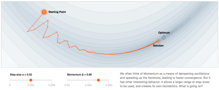
• Across the valley: The gradient components perpendicular to the valley floor flip their sign at each step. By averaging them, the momentum term dampens these oscillations.
• Along the valley: The gradient components pointing towards the minimum have a consistent sign. The momentum term accumulates these components, accelerating movement in the correct direction.

The following image illustrates this behavior. The momentum-based path is smoother and more direct than the zigzagging path of simple gradient descent we saw previously.

2. The Mathematics of Acceleration

The heavy ball analogy is useful, but the true power of momentum is revealed through a more formal analysis. In the last lesson, we saw that for an ill-conditioned quadratic, the convergence rate of gradient descent is dictated by the condition number $\kappa$, with the error decreasing by a factor proportional to $\frac{\kappa -1}{\kappa +1}$ at each step. For large $\kappa$, this is very close to 1, signifying slow convergence.

Momentum dramatically improves this. For the same problem, with optimally chosen parameters, the error decreases by a factor proportional to $\frac{\sqrt{\kappa }-1}{\sqrt{\kappa }+1}$. The "square root" improvement on the condition number is the mathematical essence of acceleration.

Professor Gilbert Strang provides a clear derivation of this result in his MIT lecture. He shows how to analyze the momentum update by converting the second-order recurrence relation into a system of two first-order equations, a standard technique you'll recognize from solving linear ordinary differential equations.

The analysis boils down to choosing the step size $\alpha$ and momentum $\mu$ to make the eigenvalues of the iteration matrix $R$ as small as possible, across all eigenvalues of the Hessian. This is a non-trivial minimax problem. The following article presents the solution and provides a rich interactive environment to explore the results.

3. Nesterov Accelerated Gradient (NAG): Looking Before You Leap

While powerful, classical momentum has a subtle flaw. It calculates the gradient at the current position $w_t$ and then adds this to the scaled velocity vector $\mu v_{t-1}$. This is like taking a big step in the direction of your accumulated momentum and, separately, a small step in the direction of the local gradient, then adding them up.

Nesterov's key insight was that it is more efficient to first use the momentum to "look ahead" to an approximate future position and then compute the gradient at that future position to make a correction. This is the "look before you leap" principle.

The update proceeds in two conceptual steps:

1. Look-ahead: Make a provisional update using only the accumulated momentum: ${\tilde{w}}_t=w_t+\mu v_{t-1}$.
2. Correction: Compute the gradient at this look-ahead point, $\nabla f({\tilde{w}}_t)$, and use it to make the final update.

This leads to the Nesterov Accelerated Gradient (NAG) update rule, in the form commonly used in deep learning (derived by Sutskever et al.):

Notice the crucial difference: the gradient is evaluated at $w_t+\mu v_{t-1}$, not at $w_t$.

Why is this better? Imagine the momentum is carrying you too far up the other side of a valley.

• Classical momentum would compute the gradient at your current position (still low in the valley), which might not strongly oppose the momentum. Only on the next step, after you've already overshot, will the gradient provide a strong correction.
• NAG would first make the momentum jump, landing high on the other side of the valley. The gradient it computes there will point sharply back towards the minimum, providing an immediate and strong braking force that corrects the overshoot before the final update is committed. This results in smaller, more efficient "U-turns."

The following video provides an excellent visual demonstration of this effect.

4. Deriving the Common Form of NAG

The common implementation of NAG, as we've seen, looks very similar to classical momentum, with the gradient evaluated at a "look-ahead" point. You may wonder how this relates to Nesterov's original formulation, which appears quite different. The following reading provides a detailed walk-through, showing how the more intuitive Sutskever formulation can be derived from the original by simply shifting the perspective of what constitutes an "iteration". Given your background, following this derivation will provide a solid understanding of the algorithm's structure.

Conclusion

In this lesson, we have moved beyond simple gradient descent to algorithms that are far more effective in the challenging, ill-conditioned landscapes of deep learning.

Key Takeaways:

• Classical Momentum introduces a "velocity" term, an exponentially weighted average of past gradients. This helps dampen oscillations across narrow valleys and builds speed along them.
• Nesterov Accelerated Gradient (NAG) improves on momentum by using the velocity term to "look ahead" before computing the gradient. This allows for a more responsive correction that reduces overshooting and leads to more stable convergence.
• The primary theoretical advantage of these methods is their improved convergence rate on ill-conditioned problems. The dependence on the condition number is reduced from $\kappa$ to $\sqrt{\kappa }$, a significant acceleration.
• There are multiple, mathematically equivalent formulations of NAG. Understanding how they relate, particularly the Sutskever "look-ahead" form, is key to its practical implementation and intuition.

We have now seen how to accelerate optimization by using a running average of the gradients (the first moment). However, all parameters in our model still share the same, global learning rate $\alpha$. What if some parameters need to move faster than others? In our next lesson, we will introduce the Adam optimizer, which combines the momentum concept with adaptive, per-parameter learning rates by tracking not only the first moment of the gradients but also the second.