Matrix Calculus for VAEs and Normalizing Flows

1. Warm-up: Linear and Quadratic Forms

Before tackling the more complex identities, let's begin with two foundational derivatives that appear frequently in machine learning. The first is the derivative of a linear transformation, and the second is the derivative of a quadratic form. These serve as excellent entry points, as their matrix forms are direct analogues of familiar scalar derivatives.

The video below offers a clear, first-principles derivation for both. The presenter starts by expanding the matrix operations into their scalar components for a 2x2 case, computes the partial derivatives to form the Jacobian, and then reveals the elegant, compact matrix result.

Let's summarize the key results. Using numerator layout (where the gradient is a column vector), we have:

• Derivative of a linear transformation: For a constant matrix $\mathbf{A}$ and a vector $\mathbf{x}$, the Jacobian of the function $f(\mathbf{x})=\mathbf{Ax}$ is $\mathbf{A}$. The gradient with respect to $\mathbf{x}$ is written as:

  $${\nabla }_{\mathbf{x}}(\mathbf{Ax})={\mathbf{A}}^T$$

  (Note: The video result is $\mathbf{A}$, which is the Jacobian matrix. When we speak of the gradient ${\nabla }_{\mathbf{x}}$ of a vector-valued function, we often mean the transpose of the Jacobian, which is consistent with the chain rule convention we've been using, ${\nabla }_{\mathbf{x}}L=J^T{\nabla }_{\mathbf{y}}L$. The distinction is subtle but important in formal settings.)

• Derivative of a quadratic form: For a symmetric matrix $\mathbf{A}$, the gradient of the scalar function $f(\mathbf{x})={\mathbf{x}}^T\mathbf{Ax}$ is:

  $${\nabla }_{\mathbf{x}}({\mathbf{x}}^T\mathbf{Ax})=2\mathbf{Ax}$$

  This identity is fundamental to the analysis of the multivariate Gaussian distribution and in deriving solutions to linear regression (Normal Equations).

2. The Main Event: Derivative of the Log-Determinant

We now arrive at the core identity for this lesson, one that is central to both Normalizing Flows and VAEs: the derivative of the logarithm of a determinant.

First, why is this important? In many generative models, we need to evaluate the probability of data under a transformation. The change of variables formula for probability densities involves the determinant of the Jacobian of the transformation. Since we typically work with log-probabilities for numerical stability and easier optimization, the term $\log |\det (\mathbf{J})|$ naturally appears in the loss function. To train the model, we must differentiate this term with respect to the model parameters.

The following video provides an excellent derivation of the identity $\frac{d}{dx}(\det (\mathbf{A}(x)))$, which we can then easily adapt for the log-determinant. The presenter uses two approaches: a direct calculation for the 2x2 case, and a more general, elegant proof using the matrix logarithm. Given your background, you will likely appreciate the second approach.

The video establishes the formula, known as Jacobi's formula:

From here, deriving the gradient for the log-determinant is a simple application of the chain rule. Let $f(\mathbf{A})=\log \det \mathbf{A}$.

Substituting Jacobi's formula for $d(\det \mathbf{A})$:

From the relationship $df=\text{tr}(({\nabla }_{A}f{)}^{T}dA)$, we can identify the gradient of $\log \det \mathbf{A}$ with respect to the matrix $\mathbf{A}$ itself.

The MIT lecture notes below formalize this result.

The key takeaway from the reading is the final identity:

If $\mathbf{A}$ is symmetric, which is often the case for covariance matrices, this simplifies to ${\nabla }_{\mathbf{A}}\log \det \mathbf{A}={\mathbf{A}}^{-1}$. This is a remarkably simple and powerful result.

3. Application to Generative Models

Let's make the connection to the papers you plan to implement explicit.

Normalizing Flows (e.g., RealNVP)

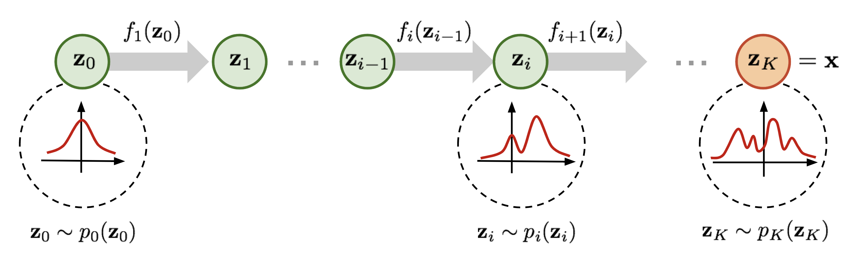
A normalizing flow models a complex data distribution $p_X(\mathbf{x})$ by transforming a simple base distribution $p_Z(\mathbf{z})$ (e.g., a standard normal) through an invertible function $\mathbf{x}=f(\mathbf{z})$. The change of variables formula dictates the resulting density:

The objective is to maximize the log-likelihood of the data, $\log p_X(\mathbf{x})$. Taking the log of the equation above, we get:

The function $f$ is a neural network with parameters $\theta$. The term $\frac{\partial f}{\partial \mathbf{z}}$ is the Jacobian of the network, $\mathbf{J}$. To train the model using gradient ascent, we must compute the gradient of the log-likelihood with respect to $\theta$. This requires us to differentiate $\log |\det (\mathbf{J}(\theta ))|$, which is a direct application of the identity we just derived.

Variational Autoencoders (VAEs)

In a VAE, we define a probabilistic encoder $q_{\varphi }(\mathbf{z}|\mathbf{x})$ and a decoder $p_{\theta }(\mathbf{x}|\mathbf{z})$. The training objective is to maximize the Evidence Lower Bound (ELBO):

Often, the encoder is chosen to be a Gaussian distribution, $q_{\varphi }(\mathbf{z}|\mathbf{x})=\mathcal{N}(\mathbf{z};\mathbf{\mu }(\mathbf{x}),\mathbf{\Sigma }(\mathbf{x}))$, where a neural network outputs the mean $\mathbf{\mu }$ and covariance $\mathbf{\Sigma }$. The prior $p(\mathbf{z})$ is typically a standard normal $\mathcal{N}(0,\mathbf{I})$.

The KL-divergence term between these two multivariate Gaussians has an analytical form which includes the term $\log \det \mathbf{\Sigma }$. Specifically:

To backpropagate the loss through the network that produces $\mathbf{\Sigma }$, we need to compute ${\nabla }_{\mathbf{\Sigma }}\log \det \mathbf{\Sigma }$, which is precisely the identity ${\mathbf{\Sigma }}^{-1}$ (assuming $\mathbf{\Sigma }$ is symmetric).

Conclusion

In this lesson, we have derived three essential matrix calculus identities and, more importantly, established their direct relevance to the mechanics of advanced generative models.

Key Takeaways:

• The derivatives of linear and quadratic forms, ${\nabla }_{\mathbf{x}}(\mathbf{Ax})={\mathbf{A}}^T$ and ${\nabla }_{\mathbf{x}}({\mathbf{x}}^T\mathbf{Ax})=2\mathbf{Ax}$, are foundational vector calculus results with direct analogues to scalar calculus.
• The gradient of the log-determinant of a matrix $\mathbf{A}$ is elegantly given by ${\nabla }_{\mathbf{A}}\log \det \mathbf{A}=({\mathbf{A}}^{-1}{)}^T$.
• This log-determinant gradient is not just a theoretical result; it is the critical component needed to optimize the log-likelihood objective in Normalizing Flows and to compute the KL-divergence term in the VAE's ELBO loss.

You now possess the specific calculus tools to understand the why behind the loss functions of these models. In our next lesson, we will synthesize what we've learned about Jacobians and gradients to trace a full backpropagation pass through a small multi-layer perceptron by hand, solidifying the mechanics of automatic differentiation.