Vector Spaces of Neural Networks

In our previous lesson, we established a geometric view of matrix multiplication, seeing it as a composition of linear transformations that warp and reshape vector spaces. This perspective is fundamental to understanding how data flows through a neural network. Today, we will build on that intuition by introducing a more formal vocabulary to describe these geometric effects.

This lesson addresses how to use vector subspaces, span, basis, and dimension to analyze the geometry of a neural network layer's weight matrix and its corresponding activation space. These concepts are not just abstract mathematical tools; they are the precise language we need to quantify a layer's expressive power, identify potential information bottlenecks, and understand what information is preserved or discarded as data is transformed.

Span, Basis, and Dimension: The Building Blocks of a Space

Before we can talk about the spaces associated with a matrix, we need to be precise about what a "space" is and how to describe it. At its core, a vector space is defined by the vectors it contains. The concepts of span, basis, and dimension give us the tools to do this efficiently.

The phenomenal "Essence of linear algebra" series by 3Blue1Brown provides the best geometric intuition for these ideas. The following video explains how vectors can be constructed from a set of "basis vectors" and what it means for a set of vectors to "span" a line, a plane, or a whole space.

Linear combinations, span, and basis vectors | Chapter 2, Essence of linear algebra

This video offers a visual and intuitive introduction to linear combinations, span, and basis vectors. As you watch, focus on building a mental model for these concepts.

Please watch the following segments: The core idea of representing vectors as linear combinations of basis vectors (like \hat{i} and \hat{j}). The definition of span: the set of all possible vectors you can reach with a linear combination of a given set of vectors. Notice how two vectors can span a line (if collinear) or an entire 2D plane. Extending to 3D, this part explains linear dependence and independence. A vector is linearly dependent on others if it's already in their span (i.e., it's redundant). A set of vectors is linearly independent if each one adds a new dimension to the span. The technical definition of a basis: a set of linearly independent vectors that span the entire space.

With that intuition in place, Professor Gilbert Strang's lecture provides a complementary, slightly more formal walkthrough. His approach, which you'll likely find familiar from your mathematics background, connects these ideas directly to matrices and their columns.

Independence, Basis, and Dimension

This lecture clip concisely defines independence, basis, and dimension. It's an excellent "working mathematician's" summary of these core concepts.

Watch these key moments: Independence and Span: Prof. Strang introduces two independent vectors and describes how their combinations "span" a plane. Defining a Basis: He defines a basis for that plane as the two vectors that are both independent and span the plane. He also introduces a third, dependent vector to show why it wouldn't be part of the basis. Spanning a Higher-Dimensional Space: An independent third vector is added to form a basis for all of \mathbb{R}^3. Formal Definition of Independence: This links independence to the null space of a matrix. The columns of A are independent if the only solution to A\mathbf{v} = \mathbf{0} is the trivial solution \mathbf{v} = \mathbf{0}. Formal Definition of Basis: A basis is a set of independent vectors that span the space. Dimension: The dimension of a space is the number of vectors in any basis for that space. This number is unique. Example with a Plane: He reinforces that a plane embedded in \mathbb{R}^3 is a two-dimensional subspace, as any basis for it will have exactly two vectors.

To summarize these crucial definitions:

Span: The set of all possible vectors that can be formed by a linear combination of a set of vectors ${v_{1}, \dots, v_{k}}$ .
Linear Independence: A set of vectors is linearly independent if no vector in the set can be written as a linear combination of the others. Formally, the only solution to $\sum c_{i} v_{i} = 0$ is $c_{i} = 0$ for all $i$ .
Basis: A set of vectors for a space (or subspace) that is both linearly independent and spans the space. A basis is a "minimal" spanning set.
Dimension: The number of vectors in a basis for a space. This number is an intrinsic property of the space itself.

The Subspaces of a Weight Matrix

Now, let's apply these concepts to a matrix $W$ , which could represent the weights of a linear layer in a neural network. A matrix transformation $y = W x$ maps vectors from an input space to an output space. The geometry of this mapping is entirely described by subspaces associated with $W$ . For this lesson, we will focus on two of the most important ones: the column space and the null space.

The Column Space: The Activation Space

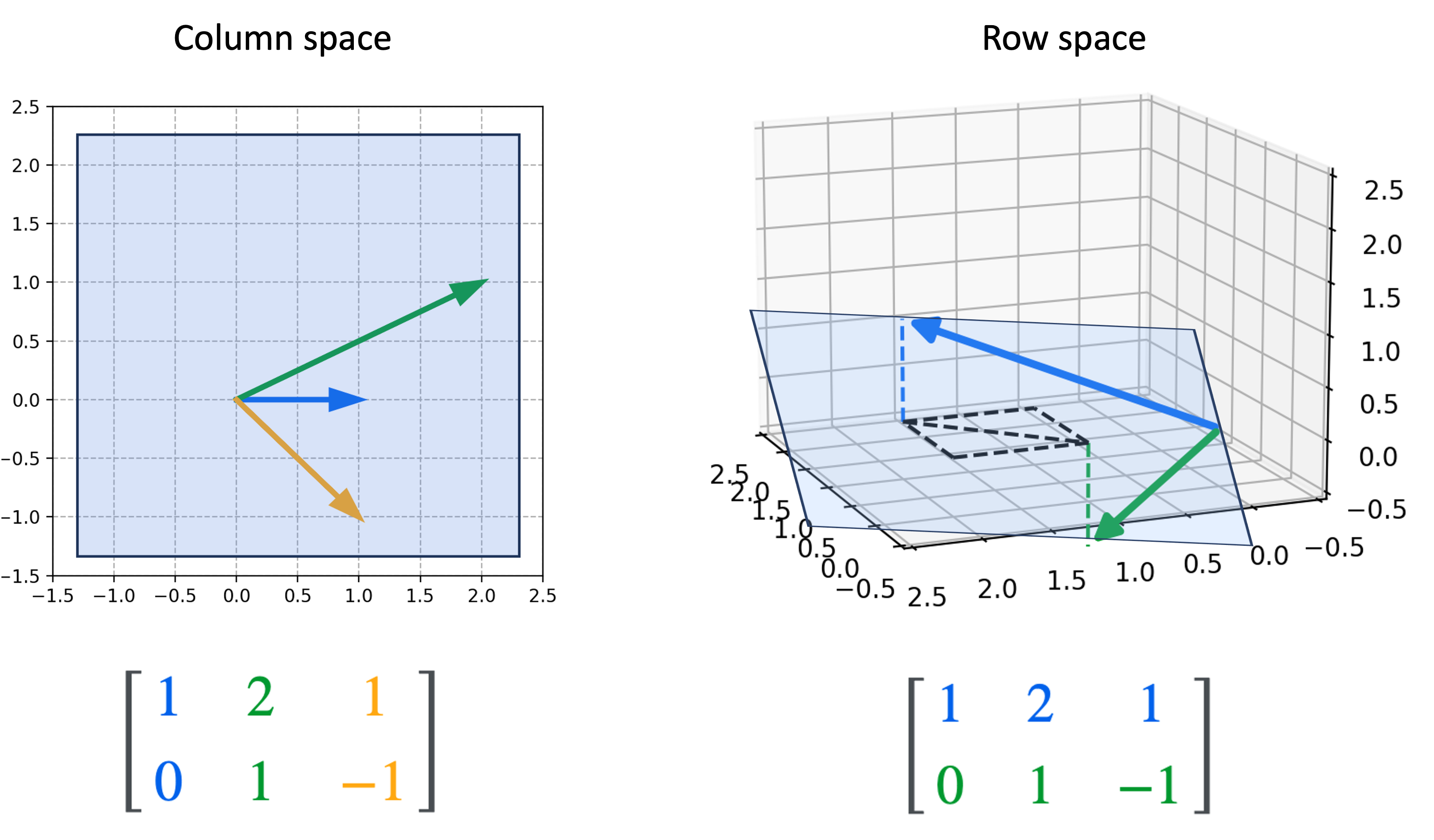
The column space of a matrix $W$ , denoted $C (W)$ , is the span of its column vectors. Why is this important? Recall from our first lesson that the product $W x$ can be interpreted as a linear combination of the columns of $W$ , where the coefficients are the elements of $x$ :

W x = ∣ w_{1} ∣ \dots ∣ w_{n} ∣ x_{1} ⋮ x_{n} = x_{1} w_{1} + \dots + x_{n} w_{n}

This means the output vector $y = W x$ is always a linear combination of the columns of $W$ . Therefore, the set of all possible outputs—the entire space of achievable activations for that layer—is precisely the column space of the weight matrix.

The dimension of the column space is called the rank of the matrix. It tells you the effective number of dimensions of the output space.

The following resource from 3Blue1Brown's website provides a clear definition of the column space and rank.

Inverse matrices, column space, and null space - 3Blue1Brown

This text clearly explains the geometric meaning of the column space and how it relates to the rank of a transformation.

Please read the section titled Column Space. Focus on the definition: the column space is the span of the matrix's columns. Also, note the connection to rank: the rank is the dimension of the output space (the column space).

If a weight matrix $W \in R^{m \times n}$ maps from an $n$ -dimensional space to an $m$ -dimensional space, but its rank is $r < m$ , the transformation is squishing the data into a lower-dimensional subspace of the target space. This creates an information bottleneck. The layer's outputs are constrained to lie on an $r$ -dimensional plane (or hyperplane) within the $m$ -dimensional ambient space.

This image visualizes the subspaces for a 2x3 matrix. The columns are 2D vectors, and their span (the column space, left) is a 2D plane. The rows are 3D vectors, and their span (the row space, right) is a 2D plane within 3D space. For this matrix, the rank is 2.

The Null Space: The Information That Is Lost

The null space (or kernel) of a matrix $W$ , denoted $N (W)$ , is the set of all input vectors $x$ that are mapped to the zero vector: $W x = 0$ .

Why does this matter for deep learning? If a non-zero input vector $x$ is in the null space, it means the specific combination of features represented by $x$ is completely "lost" or "ignored" by the linear layer. The transformation is not injective (one-to-one), because both the zero vector and $x$ map to the same output. A non-trivial null space signifies a loss of information.

Let's return to the 3Blue1Brown text to get a visual understanding of the null space.

Inverse matrices, column space, and null space - 3Blue1Brown

This section gives a great visual intuition for the null space.

Read the section titled Null Space. It explains that for transformations that are not "full rank", a whole set of vectors can be squished onto the origin. This set is the null space. The definition is clearly stated here.

Synthesis: The Geometry of a Linear Layer

Let's synthesize these ideas using a textual resource that discusses them in the context of matrices and transformations.

22.1. Geometry and Linear Algebraic Operations

This chapter from the "Dive into Deep Learning" book provides concise definitions that tie these geometric concepts together.

First, briefly review how a matrix transforms a space in Section 22.1.4. This reinforces that a matrix transforms the entire coordinate grid, and its action is fully determined by where it sends the basis vectors. Next, read Section 22.1.5 on Linear Dependence. It shows how a linear dependence in the columns of a matrix, like \mathbf{b}_1 = -2\mathbf{b}_2, is evidence that the matrix compresses the space to a lower dimension. Finally, read Section 22.1.6 on Rank. It formally defines rank as the maximum number of linearly independent columns. This number is exactly the dimension of the column space.

In the context of a linear layer with weight matrix $W$ :

The column space $C (W)$ is the activation space—the set of all possible outputs.
The rank, $rank (W) = dim (C (W))$ , is the dimension of this activation space. If the rank is less than the number of rows in $W$ , the layer acts as an information bottleneck.
The null space $N (W)$ is the set of input features that are discarded by the layer. Its dimension is called the nullity.

These concepts give you a powerful geometric toolkit. When you see a nn.Linear(in_features=512, out_features=128) layer, you can now think of its weight matrix not just as a table of numbers, but as a map from a 512-dimensional space to a 128-dimensional subspace. The rank of this matrix tells you the true dimensionality of the information being passed forward, and its null space tells you what's being left behind.

Conclusion

In this lesson, we developed a formal language to describe the geometry of linear transformations, which are the building blocks of neural networks.

Key Takeaways:

Span, Basis, and Dimension are the fundamental concepts for describing vector spaces. A basis is a minimal, independent set of vectors that spans the entire space, and its size gives the space's dimension.
The Column Space of a weight matrix $W$ is the span of its columns. It represents the "activation space"—the set of all possible outputs of the linear layer. Its dimension is the rank of $W$ .
A rank deficient matrix (where rank is less than the number of rows) creates an information bottleneck, projecting the data into a lower-dimensional subspace.
The Null Space of $W$ is the set of all input vectors that map to zero. It represents the information that is discarded by the layer.

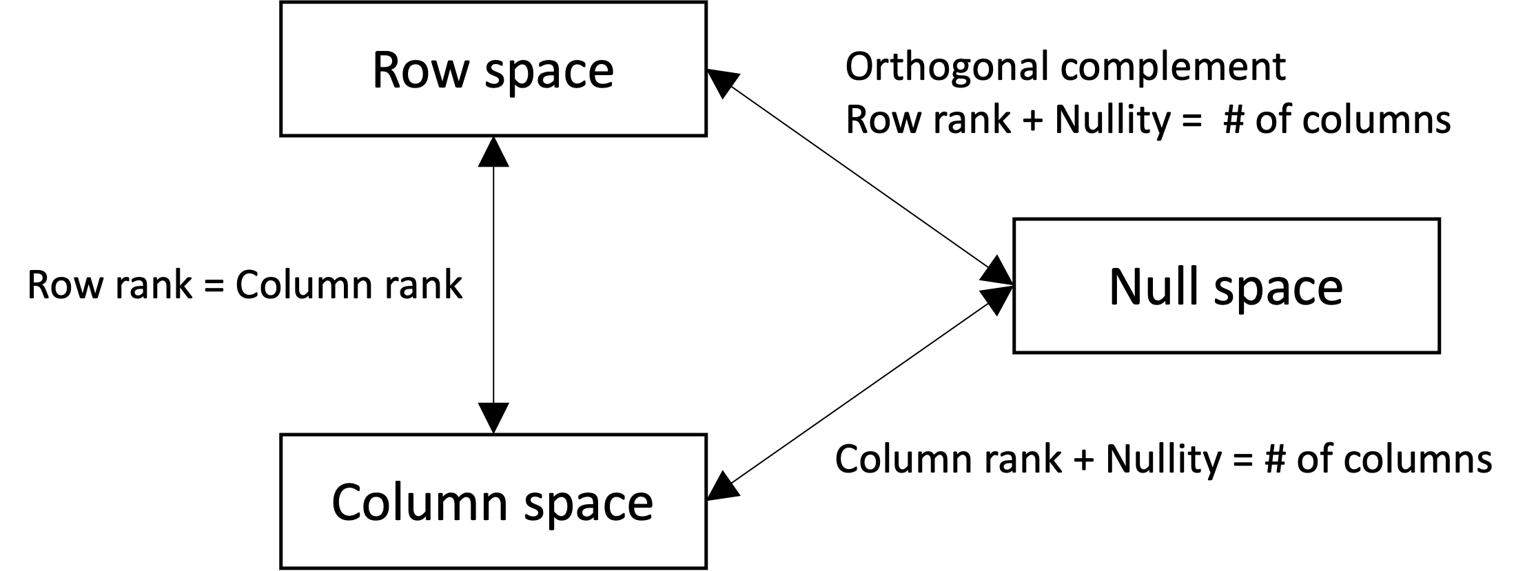
This diagram shows the relationships between the fundamental subspaces. We've explored the Column Space and Null Space, and their connection to rank.

In our next lesson, we will complete this picture by analyzing all four fundamental subspaces of a matrix, including the row space and left null space. We will explore the deep and elegant orthogonal relationships between them, which will directly lead us to understanding crucial techniques like least-squares approximation and data preprocessing.