Orthogonal Projections, Least Squares, and Data Whitening

Orthogonal Projection: Finding the Closest Point

At its heart, projection is about simplification. When we project a vector $\mathbf{b}$ onto a subspace, we are finding the vector $\hat{\mathbf{b}}$ within that subspace that is closest to $\mathbf{b}$. The "error" of this approximation, the vector $\mathbf{e}=\mathbf{b}-\hat{\mathbf{b}}$, is orthogonal to the subspace itself.

The geometry of projection provides a powerful way to solve problems where an exact solution doesn't exist. To build the machinery, we will derive the formula for a projection matrix step-by-step, starting from the simplest case and building to the general one.

The following video provides an exceptionally clear, bottom-up derivation of the projection matrix formulas. It moves from projecting onto a single vector to projecting onto a general subspace, which is exactly the tool we need.

Let's summarize the crucial result from the video. To project a vector $\mathbf{b}$ onto the column space of a matrix $A$, we must find the point $\hat{\mathbf{b}}=A\hat{\mathbf{x}}$ in $C(A)$ such that the error vector $\mathbf{e}=\mathbf{b}-\hat{\mathbf{b}}$ is orthogonal to $C(A)$. As we learned last lesson, being orthogonal to the column space means being in the left null space, $N(A^T)$.

This gives us the core condition:

Rearranging this gives the celebrated normal equations:

Solving for $\hat{\mathbf{x}}$ gives the coordinates of the projection in the basis defined by $A$. The projection vector itself is $\hat{\mathbf{b}}=A\hat{\mathbf{x}}$.

If $A^{T}A$ is invertible, we can write:

And the projection is:

This defines the projection matrix $P$ that maps any vector $\mathbf{b}$ to its projection $\hat{\mathbf{b}}$ in $C(A)$:

Application: The Geometry of Least Squares

The framework of orthogonal projection provides the most elegant derivation of the solution to the least squares problem. Consider an overdetermined system $A\mathbf{x}=\mathbf{b}$, common in data science, where you have more equations (observations) than unknowns. In this case, $\mathbf{b}$ is typically not in the column space of $A$, so no exact solution exists.

The goal is to find the "best" approximate solution, $\hat{\mathbf{x}}$, which minimizes the length of the error vector $||\mathbf{e}||=||A\mathbf{x}-\mathbf{b}||$. Geometrically, this minimum is achieved precisely when $A\hat{\mathbf{x}}$ is the orthogonal projection of $\mathbf{b}$ onto $C(A)$.

Therefore, solving the least squares problem is equivalent to solving the normal equations.

Professor Strang's lecture provides an excellent walkthrough of this connection. He masterfully switches between the two pictures of least squares: the data-fitting view with points and lines, and the vector space view with projections.

An essential technical point is the invertibility of the matrix $A^{T}A$. If this matrix isn't invertible, a unique least squares solution doesn't exist. This happens if the columns of $A$ are linearly dependent.

Professor Strang provides a concise proof that if the columns of $A$ are linearly independent (which is the case when they form a basis for the column space), then $A^{T}A$ is guaranteed to be invertible. This is a key theoretical underpinning for least squares.

Data Decorrelation and Whitening

We've seen how projections help solve systems. Now, let's see how related geometric transformations are used to preprocess data. In many machine learning algorithms, particularly older ones but also as a component in modern architectures, performance is improved if the input features are uncorrelated and have similar variance.

Let's represent our dataset as a matrix $X\in {\mathbb{R}}^{n\times d}$, where $n$ is the number of samples and $d$ is the number of features. We assume the data is centered, meaning the mean of each feature (column) has been subtracted.

The sample covariance matrix is then given by $S=\frac{1}{n-1}{X}^{T}X$. The diagonal entries of $S$ are the variances of the features, and the off-diagonal entries are the covariances.

1. Decorrelation: Our goal is to transform the data such that the new features are uncorrelated. This is equivalent to making the new covariance matrix diagonal. This is precisely what Principal Component Analysis (PCA) achieves. The principal components are the eigenvectors of the covariance matrix $S$. Projecting the data onto these eigenvectors rotates the data to align with its axes of principal variance, which by construction are orthogonal.

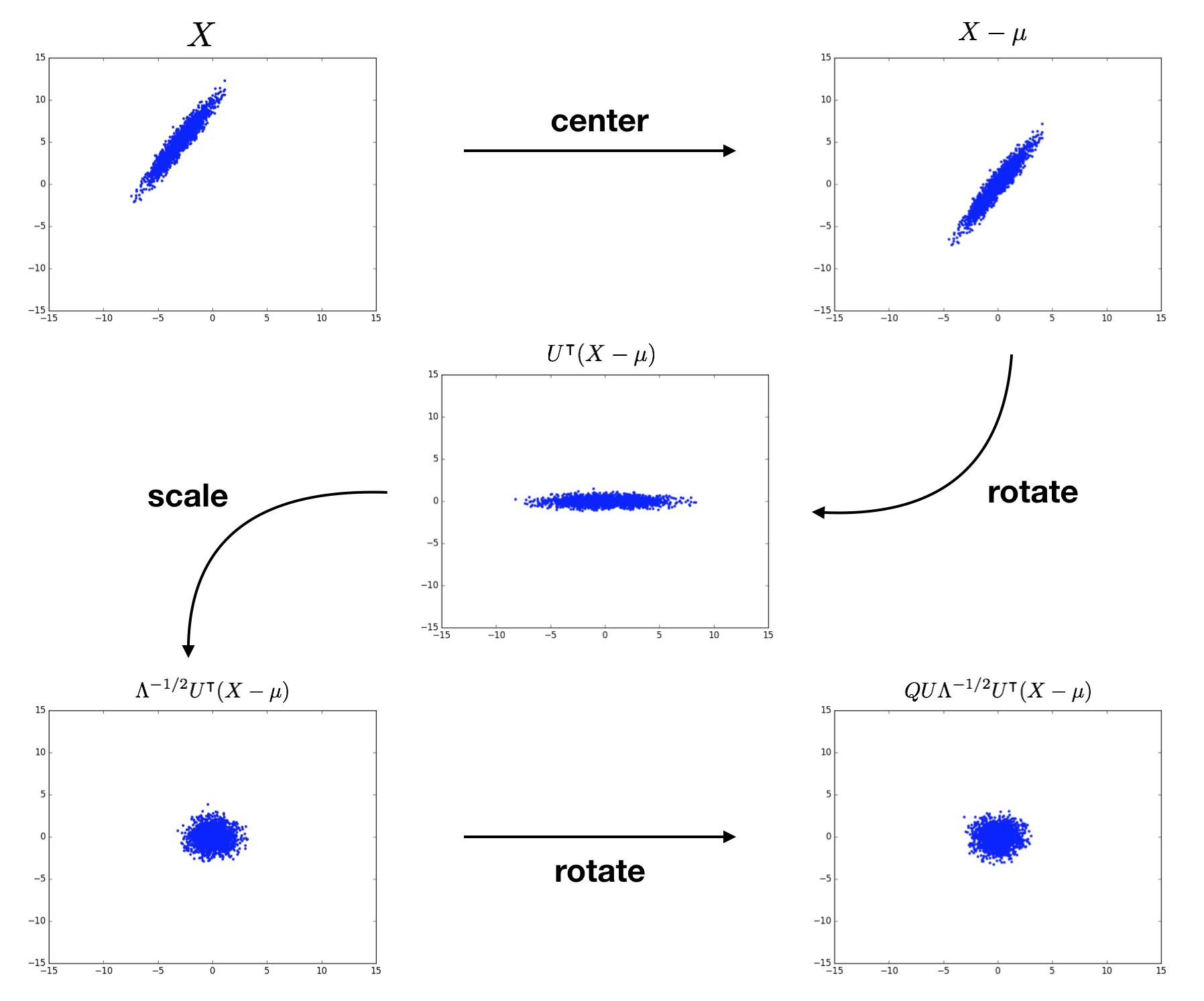
2. Whitening: Whitening takes this one step further. It not only decorrelates the data but also scales it so that each feature has a variance of 1. The resulting covariance matrix is the identity matrix, $I$. Geometrically, if the original data forms an elliptical cloud, whitened data forms a spherical cloud. This process is also known as "sphering" the data.

The sequence of transformations to achieve whitening is shown beautifully in the following diagram.

There are two main types of whitening:

• PCA Whitening: After rotating the data $X$ onto its principal axes (given by the right singular vectors $V$ of $X$), we get scores $T=XV$. We then scale each new feature by the inverse of its standard deviation (the singular values ${\sigma }_i$). The full transformation is $X_{\text{PCA-white}}=XV{\Sigma }^{-1}$, where $\Sigma$ is the diagonal matrix of singular values of $X$. The new covariance matrix is indeed $I$.

• ZCA Whitening: PCA whitening can drastically change the data by rotating it. ZCA (Zero-phase Component Analysis) whitening aims to whiten the data while staying as close as possible to the original. It achieves this by applying the inverse of the PCA rotation after whitening.

  $$X_{\text{ZCA}}=X_{\text{PCA-white}}{V}^T=(XV{\Sigma }^{-1})V^T=X(V{\Sigma }^{-1}{V}^T)$$

  You may see this written as $X{S}^{-1/2}$, where $S^{-1/2}$ is the inverse square root of the covariance matrix. This form is common in deep learning literature, for example, as a theoretical basis for some optimizer or normalization techniques.

The image below compares the result of these two transformations.

Conclusion

In this lesson, we explored the practical power of orthogonality through the lens of projections.

Key Takeaways:

• Orthogonal projection finds the closest point in a subspace to a given vector. The projection matrix $P=A(A^{T}A{)}^{-1}{A}^T$ projects vectors onto the column space of $A$.
• The least-squares solution to an inconsistent system $A\mathbf{x}=\mathbf{b}$ is found by solving the normal equations $A^{T}A\hat{\mathbf{x}}=A^T\mathbf{b}$, which is a direct consequence of orthogonal projection.
• Decorrelation and whitening are crucial data preprocessing steps that simplify a dataset's statistical properties. They transform a correlated, anisotropic data cloud into an uncorrelated (diagonal covariance) or spherical (identity covariance) one.
• These transformations are fundamentally geometric operations—rotations and scalings—revealed by the eigendecomposition of the covariance matrix or the SVD of the data matrix.

We are building a powerful geometric vocabulary. So far, we have seen how linear maps can be decomposed into rotations and scalings, and how we can use this to understand information flow, solve systems, and transform data distributions.

In our next lesson, we will add another layer to our understanding by exploring determinants and traces. We will see how determinants measure the change in volume induced by a linear transformation, a concept that is not just a theoretical curiosity but a critical component in one of your target implementations: Normalizing Flows.