Welcome to your first lesson. We'll begin by diving into one of the most fundamental concepts in machine learning: the bias-variance tradeoff. Understanding this principle is crucial because it explains why a model might perform brilliantly on the data it was trained on, yet fail when faced with new, unseen data. For any application, especially in a high-stakes environment like fintech, building models that are not just accurate but also reliable and generalizable is paramount. This lesson will provide the conceptual framework for why that's a challenging balancing act.
By the end of this lesson, you will be able to explain the bias-variance tradeoff and how it relates directly to a model's complexity, a topic that frequently comes up in ML interviews.
The Intuition: Accuracy vs. Precision
Before we get into the formal definitions, let's build some intuition. Imagine you are at a shooting range. Your goal is to hit the bullseye. The bias-variance tradeoff can be visualized using this analogy.

*This image provides a classic analogy for bias and variance.
- Low Bias, Low Variance (Top-Left): Your shots are tightly clustered around the bullseye. This is the ideal scenario. Your predictions are, on average, correct (low bias) and consistent (low variance).
- Low Bias, High Variance (Top-Right): Your shots are centered around the bullseye, but they are spread out. On average, you're getting it right, but individual shots are unreliable. This model is sensitive to small changes in the data.
- High Bias, Low Variance (Bottom-Left): Your shots are tightly clustered but miss the bullseye. Your model is consistent but systematically wrong. It has failed to capture the true underlying relationship.
- High Bias, High Variance (Bottom-Right): Your shots are spread out and miss the bullseye. The model is neither accurate nor consistent. This is the worst-case scenario.*
In machine learning:
- Bias is a measure of a model's systematic error. High bias means the model makes strong, often simplistic, assumptions about the data, leading it to miss the true relationship between inputs and outputs. This is often called underfitting.
- Variance is a measure of how much a model's predictions would change if you were to train it on a different training dataset. High variance means the model is overly sensitive to the noise and specific patterns in its training data. This is known as overfitting.
To solidify this intuition, let's watch a short, clear explanation.
Machine Learning Fundamentals: Bias and Variance
This video from StatQuest provides an excellent and memorable walkthrough of bias and variance using a simple example.
Watch the entire video. Pay close attention to how the "straight line" model represents high bias and low variance, while the "squiggly line" represents low bias and high variance. Notice the distinction between performance on the training set versus the testing set.
Model Complexity: Underfitting and Overfitting
As the video demonstrated, the complexity of a model is at the heart of the bias-variance tradeoff. A simple model, like linear regression, might not be flexible enough to capture a complex, non-linear pattern (high bias). A highly complex model, like a deep decision tree or the "squiggly line," can fit the training data almost perfectly but may learn the noise instead of the signal, leading to poor performance on new data (high variance).
Let's explore this interactively.
Bias Variance Tradeoff - MLU-Explain
This interactive article provides a fantastic visual demonstration of how model complexity leads to underfitting and overfitting.
Please read through the first few sections of the article. Start from the beginning and read the introduction. Continue to the section on underfitting. Observe how the simple linear model fails to capture the curve, resulting in high error on both training and test data. Next, review the section on overfitting. See how the complex model perfectly fits the training data (zero training error) but performs poorly on the test data because it has memorized the noise.
This dynamic between training error and test error is a classic sign of where your model lies on the complexity spectrum. The article "Mastering the Bias-Variance Tradeoff" provides a concise table that is perfect for interview preparation.
Mastering the Bias-Variance Tradeoff in Machine Learning
This section from a blog post by Lightly AI clearly summarizes the differences between underfitting and overfitting.
Find the section titled "Underfitting vs Overfitting: Too Simple vs Too Complex Models". Focus on the table, which neatly contrasts the two conditions across model complexity, error types, bias, variance, and potential fixes.
The Mathematical Foundation of Error
So far, we've established that a model's error on unseen data is influenced by both bias and variance. Machine learning theory formally decomposes this error. The expected error of any predictive model on a new data point can be broken down into three components:
- Bias²: The squared difference between the average prediction of our model and the true value we are trying to predict. It measures how far off the model's average prediction is from the correct value.
- Variance: The variability of a model prediction for a given data point. It measures how much the predictions would vary if we were to train the model on different random subsets of the data.
- Irreducible Error (Noise): This error comes from the inherent randomness or noise in the data itself. No matter how good our model is, we cannot eliminate this error. It represents a theoretical lower bound on the error.
Given your background in engineering, you might appreciate a more formal derivation. The following video from the Stanford Statistical Learning course provides exactly that.
Statistical Learning: 2.3 Model Selection and Bias Variance Tradeoff
This excerpt from a lecture by Prof. Trevor Hastie, one of the authors of the seminal textbook "An Introduction to Statistical Learning," provides the mathematical decomposition of prediction error.
Watch the segment from the derivation. Focus on how the expected prediction error is broken down into variance, bias, and the irreducible error. Don't worry about memorizing the derivation, but aim to understand what each of the three terms represents conceptually.
Visualizing the Tradeoff
The relationship between bias, variance, and model complexity results in a characteristic U-shaped curve for the total error. This is perhaps the most important visualization related to this topic.
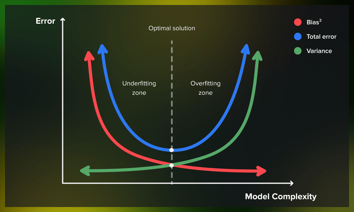
This graph shows how error components change with model complexity. As complexity increases, bias (red curve) decreases because the model becomes more flexible and can fit the training data better. However, variance (green curve) increases as the model starts fitting the noise in the training data. The total error (blue curve) is the sum of these components, and it reaches a minimum at an optimal level of complexity, often called the "sweet spot".
Your goal as a machine learning engineer is to find a model that operates in this sweet spot, balancing the two sources of reducible error.
- To the left of the sweet spot: The model is too simple (e.g., linear regression for a complex problem). It is underfitting, suffering from high bias.
- To the right of the sweet spot: The model is too complex (e.g., an unpruned decision tree). It is overfitting, suffering from high variance.
Many machine learning algorithms have "hyperparameters" that allow you to control model complexity and navigate this tradeoff. For example, in a K-Nearest Neighbors (KNN) algorithm, the value of K directly controls complexity. A small K leads to a very flexible (high-variance) model, while a large K leads to a very smooth, rigid (high-bias) model.
Key Takeaways
To conclude, let's summarize the key points you should be ready to articulate in an interview:
- Total prediction error on unseen data is a combination of bias, variance, and irreducible error. Our goal is to minimize the sum of bias and variance.
- Bias arises from a model's overly simple assumptions, causing it to miss the true underlying patterns (underfitting). High-bias models are systematically inaccurate.
- Variance arises from a model's excessive sensitivity to the training data, causing it to learn noise (overfitting). High-variance models are inconsistent and don't generalize well.
- The Bias-Variance Tradeoff: There is an inverse relationship between bias and variance. Increasing a model's complexity typically decreases bias but increases variance.
- Model Complexity: The central challenge is to find the optimal model complexity that balances this tradeoff to achieve the lowest possible error on new, unseen data. This is visualized by the U-shaped total error curve.
In our next lesson, we will explore regularization (L1 and L2). Regularization techniques are a powerful and widely used set of tools designed specifically to manage this tradeoff by constraining a model's complexity, thereby helping to prevent overfitting.