Understanding Logistic Regression: Probability and Decision Boundaries

From Linear Regression to Classification

Let's start by considering why we can't just use the linear regression models we've been discussing for a classification task, like predicting whether a financial transaction is fraudulent (1) or not (0).

A linear model, $y={\theta }^{T}x$, outputs a value that can range from $-\infty$ to $+\infty$. This is problematic for two reasons:

1. The output doesn't conform to a probability, which must lie between 0 and 1.
2. In a binary {0, 1} setting, an output of, say, 3 or -0.5 has no intuitive meaning.

This is the core problem logistic regression is designed to solve. It elegantly adapts the linear model framework to produce a valid probability. The video below provides a concise explanation of this transition.

Modeling Probability with the Sigmoid Function

The solution is to take the output of the linear equation, $z={\theta }^{T}x$, and pass it through a function that "squashes" the entire real number line into the (0, 1) interval. This function is the sigmoid function, also called the logistic function.

The sigmoid function is defined as:

Here, $z$ is the output of our linear model, ${\theta }_0+{\theta }_1{x}_1+\cdots +{\theta }_n{x}_n$. The result, $\sigma (z)$, is a number between 0 and 1, which we can interpret as the probability that the given input $x$ belongs to the positive class (y=1).

So, the hypothesis of our logistic regression model is:

The video below by Emma Ding provides an exceptionally clear, two-step summary of this process, which is a great framework for an interview explanation.

To solidify these concepts, let's turn to a more detailed textual resource.

From Probability to a Decision Boundary

Now that our model outputs a probability, how do we make a final classification? We apply a decision rule. The most common rule is to set a threshold at 0.5:

• If $h_{\theta }(x)\ge 0.5$, we predict class 1.
• If $h_{\theta }(x)<0.5$, we predict class 0.

This simple threshold has a profound geometric meaning. Let's look at the sigmoid function's graph. You'll notice that $\sigma (z)\ge 0.5$ whenever its input $z\ge 0$. Since our input is $z={\theta }^{T}x$, our decision rule becomes:

• Predict 1 if ${\theta }^{T}x\ge 0$.
• Predict 0 if ${\theta }^{T}x<0$.

The equation ${\theta }^{T}x=0$ defines the decision boundary. This is the surface (a line in 2D, a plane in 3D, a hyperplane in higher dimensions) that separates the feature space into two regions: the "predict 1" region and the "predict 0" region. It is a linear boundary because the equation defining it is linear in the features $x$.

The image below, from a lecture by Andrew Ng, visualizes this exact concept.

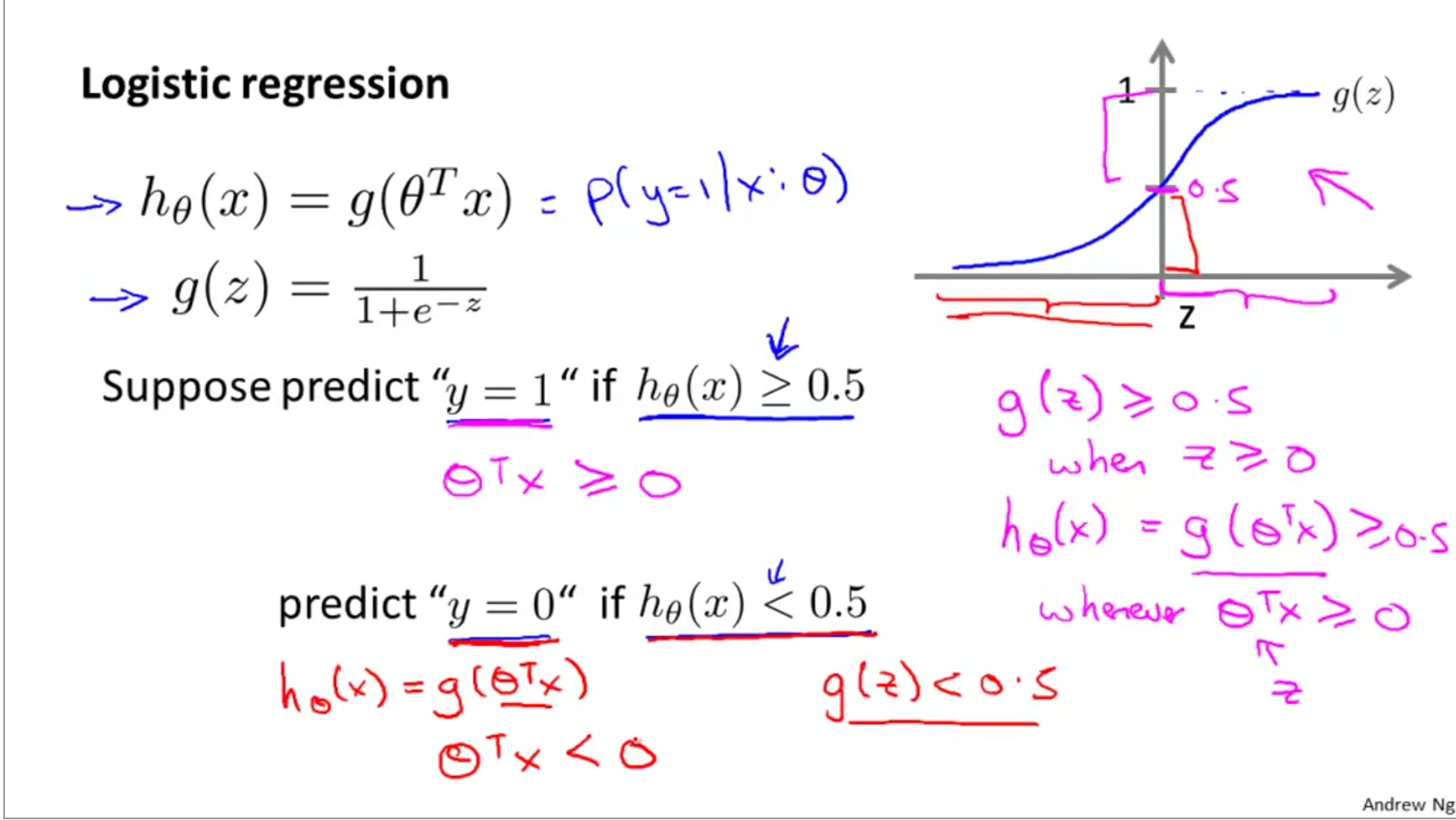
The following reading provides a much more detailed exploration with visualizations, showing how this boundary manifests in one and two dimensions.

When a logistic regression model is trained on a dataset with multiple features, this boundary separates the data points. Points on one side are classified as belonging to one class, and points on the other side to the other class.

A Note on Model Training and Regularization

How does the model find the right parameters ($\theta$) to place this boundary correctly? It's done through an optimization process called Maximum Likelihood Estimation, which aims to find the $\theta$ values that maximize the probability of observing the true labels in the training data. This is typically solved using iterative methods like Gradient Descent.

Importantly, just like linear regression, logistic regression can overfit. In our last lesson, we saw how regularization penalizes large coefficients. The same principle applies here. In fact, regularization is critical for logistic regression. If the data is perfectly separable by a line, the "optimal" coefficients can grow towards infinity to make the sigmoid curve infinitely steep, leading to an overconfident model. By adding an L1 or L2 penalty, we constrain the size of the coefficients, ensuring a more robust and generalizable decision boundary. Most standard implementations, like scikit-learn's LogisticRegression, apply L2 regularization by default.

Conclusion

In this lesson, we have deconstructed logistic regression, a cornerstone of classification. You are now prepared to explain its mechanics with the precision required for a technical interview.

Key Takeaways for Your Interview:

• Purpose: Logistic regression is a classification algorithm that models the probability of a binary outcome.
• Modeling Probability: It uses the sigmoid (or logistic) function to map the output of a linear model (${\theta }^{T}x$) to a probability between 0 and 1. This probability is $P(y=1|x)$.
• Decision Boundary: By applying a threshold (typically 0.5) to the output probability, a decision rule is created. This rule is equivalent to checking the sign of ${\theta }^{T}x$, and the equation ${\theta }^{T}x=0$ defines a linear decision boundary in the feature space.
• Linearity: It's important to remember that while logistic regression models a non-linear probability function, the decision boundary it produces is linear.

In our next lesson, we will explore a completely different approach to classification: decision trees. Unlike the linear models we've studied, decision trees create non-linear decision boundaries by recursively partitioning the feature space, offering a powerful alternative with different strengths and weaknesses.