Welcome back! In our last lesson, we focused on cleaning data by identifying and handling outliers, a crucial step for building robust models. We established that the right approach depends on the data's origin and the model's sensitivity, with a special emphasis on how, in fintech, an outlier might be the most important signal of all.
Today, we shift from cleaning existing data to creating entirely new information. We will explore how to engineer features from temporal data, focusing on two foundational techniques: lags and rolling windows. Standard machine learning models don't inherently understand the sequence of time. For them, a dataset is just a collection of independent rows. Your job as an engineer is to create features that explicitly encode this temporal context, transforming a time series problem into a supervised learning task that models like Gradient Boosting or Random Forests can solve. This skill is paramount in fintech for everything from forecasting market movements to modeling customer lifetime value.
Why Do Machine Learning Models Need Temporal Features?
Imagine you have daily sales data and you want to predict tomorrow's sales. If you feed a raw timestamp and a sales number to a model like a Random Forest, it has no intrinsic concept that 2023-10-26 comes directly after 2023-10-25. It can't see trends, seasonality, or momentum. We need to create features that make these patterns explicit.
This process transforms the problem from "predict the next value in a sequence" to "predict a target value given a set of features," which is the standard tabular format for supervised ML. The following video provides an excellent motivation for why this approach is so powerful.
Kishan Manani - Feature Engineering for Time Series Forecasting | PyData London 2022
This talk from PyData London by Kishan Manani clearly articulates the shift from classical time series forecasting to using ML models on engineered features.
First, watch the introduction from here, where the speaker frames the core idea of converting a time series task into a tabular regression task. Next, watch the segment from the M5 competition example. This real-world case study on Walmart sales data shows why ML models with rich feature engineering often outperform traditional statistical methods like ARIMA, especially with complex, multi-series datasets common in large enterprises.
The key takeaway is that by creating features, we give the model the context it needs to learn from the past to predict the future. Let's dive into the two most fundamental ways to do this.
Technique 1: Lag Features
Lag features are the simplest and often most powerful type of temporal feature. A "lag" is simply a value from a previous time step.
- Lag 1 for today's sales would be yesterday's sales.
- Lag 7 for daily data would be the sales from the same day last week.
These features allow the model to capture two critical patterns:
- Persistence/Momentum: The recent past is often a good predictor of the near future. If a stock was rising yesterday, it might continue today.
- Seasonality: Behavior often repeats in cycles. Retail sales have weekly patterns (weekends vs. weekdays), and financial markets can have quarterly or yearly patterns.
Data Science Interview Guide: Time Series Forecasting
This guide provides a concise, interview-focused explanation of lag features.
Read the section titled Lag Features. Pay attention to how the choice of lag (e.g., lag 7 for retail, lag 24 for hourly electricity) depends on domain knowledge of the underlying cycles in the data.
Implementation in Pandas and SQL
Creating lag features is straightforward. In Python with pandas, you use the .shift() method. In SQL, you use the LAG() window function. Notice how both achieve the same result. As you prepare for your interview, being able to articulate solutions in both paradigms is a significant strength.
Practical Guide for Feature Engineering of Time Series Data
This article provides clear, parallel code examples for creating temporal features in both pandas and SQL.
Focus on the section Lag Features. Review both the Python and SQL code blocks. Note the use of groupby().shift() in pandas to prevent data from one time series (e.g., one store) leaking into another when calculating lags. In SQL, the PARTITION BY clause serves the same purpose.
Technique 2: Rolling Window Features
While lag features look at single points in the past, rolling window features summarize a range of recent past values. You define a window size (e.g., 7 days) and then calculate a statistic (e.g., mean, standard deviation, min, max) over that sliding window.
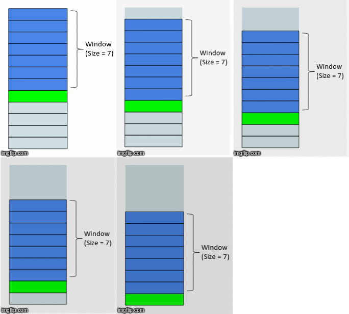
Common rolling window features include:
- Rolling Mean: Smooths out short-term noise to highlight the underlying trend. A 30-day rolling average of a stock's price is a classic trend indicator.
- Rolling Standard Deviation: Measures recent volatility. A sudden spike in the rolling standard deviation of transaction amounts could signal anomalous or fraudulent activity.
- Rolling Min/Max: Can identify recent peaks or troughs.
Implementation and the Peril of Data Leakage
Implementing rolling windows is also straightforward, using .rolling() in pandas or window frames in SQL.
Practical Guide for Feature Engineering of Time Series Data
Let's continue with the same practical guide.
Now, read section Rolling Window Statistics. Again, compare the pandas implementation using .rolling() with the SQL implementation using AVG() OVER (...) ROWS BETWEEN .... This SQL syntax is a powerful tool for analytics.
However, when creating rolling features, you must be extremely careful to avoid data leakage. Data leakage occurs when your features accidentally contain information from the future that won't be available at prediction time.
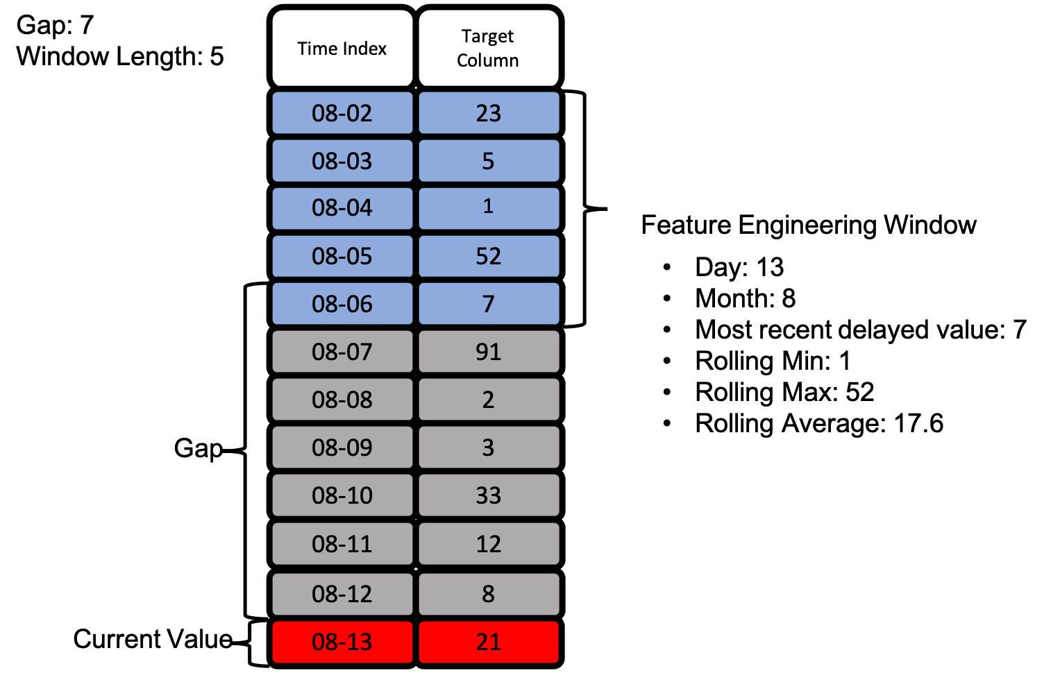
For a rolling window, the calculation for a given day must not include that day's own value. If you calculate a 7-day rolling average to predict today's sales, that average must be based on the previous 7 days, not the 6 previous days plus today.
The following image illustrates the correct setup. Notice the "Gap" between the "Feature Engineering Window" and the "Current Value." This gap ensures no future information contaminates the features.
The speaker in the PyData talk provides a sharp explanation of this common pitfall.
Kishan Manani - Feature Engineering for Time Series Forecasting | PyData London 2022
Let's return to the PyData London talk for a critical point on implementation.
Watch the segment from window features and leakage. The speaker's key point is that after you compute a rolling statistic like pd.rolling().mean(), you must then apply .shift(1) to ensure the feature for time t only contains information from t-1 and earlier. This is a subtle but crucial detail.
Other Temporal Features
Lags and rolling windows are the building blocks, but you can create many other features from a timestamp:
- Calendar Features: These are static features derived from the date itself, such as day of the week, week of the year, month, quarter, or a binary flag for holidays. These are simple to create and very effective at capturing human-driven seasonal patterns.
- Complex Features: You can combine the techniques above. For example: "the ratio of today's value to the rolling 7-day average" (a measure of current deviation from the trend) or "the average sales for the same week of the year last year" (combining lag and window features).
For an interview, being able to brainstorm such features demonstrates a deep understanding of the problem.
Conclusion
You now have a solid framework for engineering features from temporal data. This process is the bridge that allows powerful but time-agnostic ML models to excel at forecasting and sequence modeling tasks.
Key Takeaways:
- Time to Tabular: The goal of temporal feature engineering is to convert a sequence problem into a tabular format that standard ML models can use.
- Lag Features: Use past values directly with
.shift()orLAG()to capture momentum and seasonality. - Rolling Window Features: Summarize recent behavior with
.rolling()or... OVER (ROWS BETWEEN ...)to capture local trends and volatility. - Avoid Data Leakage: This is the most critical rule. Features for time must only be created from data known at or before time . Always ensure there is a "gap" between your feature window and your target.
- Domain Knowledge: The choice of lags (e.g., 7 for weekly data) and window sizes is guided by understanding the underlying process you are modeling.
In our next lesson, we will extend these ideas to a different kind of time-ordered data: transactional data. We'll see how to engineer features like RFM (Recency, Frequency, Monetary) metrics and behavioral aggregations to model customer behavior, a core task in many fintech applications.