Parallel Efficiency and Scalability

Introduction

Hello! In our last lesson, we contrasted Amdahl's Law and Gustafson's Law, revealing two distinct goals in parallel computing: solving a fixed problem faster (strong scaling) versus solving a larger problem in the same amount of time (weak scaling). These laws give us theoretical speedup limits based on a program's serial fraction.

Today, we move from theoretical limits to practical measurement. This lesson will equip you with the tools to answer the question: "How effectively is my parallel program actually using the hardware?"

Our learning outcome is to define and calculate parallel efficiency and distinguish between strong and weak scalability. We will define parallel efficiency as a key performance metric and then formalize the processes of analyzing both strong and weak scaling, which are fundamental practices in performance engineering.

1. What is Parallel Efficiency?

The most common metric for parallel performance is speedup, which we've already used. As a reminder, speedup ( $S_{P}$ ) on $P$ processors is the ratio of the best sequential execution time ( $T_{1}$ ) to the parallel execution time ( $T_{P}$ ).

S_{P} = \frac{T _{1}}{T _{P}}

Ideally, using $P$ processors would make our program run $P$ times faster, meaning $S_{P} = P$ . This is called linear speedup. In reality, factors like communication overhead, synchronization, and the unavoidable serial parts of the code prevent us from achieving this.

Parallel efficiency is a metric that quantifies how close we are to this ideal. It is defined as the ratio of the observed speedup to the ideal speedup.

To explore this concept further, let's turn to a concise definition.

Parallel Performance and Scalability – ACENET Summer School

The following resource from ACENET's Summer School provides a clear definition of what it calls 'Scalability (also referred to as efficiency)'.

Please read the short section titled 'Scalability'. Note that this resource uses the terms 'Scalability' and 'Efficiency' interchangeably. Focus on its definition and the formula it presents.

As the reading explains, the formula for parallel efficiency, $E_{P}$ , on $P$ processors is:

E_{P} = \frac{S _{P}}{P}

By substituting the formula for speedup, we get:

E_{P} = \frac{T _{1} / T _{P}}{P} = \frac{T _{1}}{P \times T _{P}}

Efficiency is typically expressed as a value between 0 and 1 (or as a percentage).

$E_{P} = 1$ (100%): Perfect linear speedup. Each processor is contributing its full potential 100% of the time.
$E_{P} < 1$ : The typical case. An efficiency of 0.75, for example, means that on average, each processor is being used effectively for 75% of the execution time. The remaining 25% is lost to parallel overhead.

2. A Worked Example

Let's make this concrete. Imagine you've parallelized a C++ simulation that originally took $T_{1} = 400$ seconds to run on a single CPU core. When you run it on a workstation with $P = 8$ cores, the execution time drops to $T_{8} = 62.5$ seconds.

Calculate the Speedup:
$S_{8} = \frac{T _{1}}{T _{8}} = \frac{400 s}{62.5 s} = 6.4 x$
The program is 6.4 times faster on 8 cores.
Calculate the Efficiency:
$E_{8} = \frac{S _{8}}{P} = \frac{6.4}{8} = 0.8$
The parallel efficiency is 80%. This is a good result, indicating that the overheads are relatively small. Only 20% of the potential computing power is being lost.

3. Strong vs. Weak Scalability: A Formal Distinction

In our previous lessons, we associated Amdahl's Law with strong scaling and Gustafson's Law with weak scaling. Now, let's formalize these as two distinct types of performance analysis. The choice between them depends entirely on your goal.

The following image provides an excellent visual intuition for the difference.

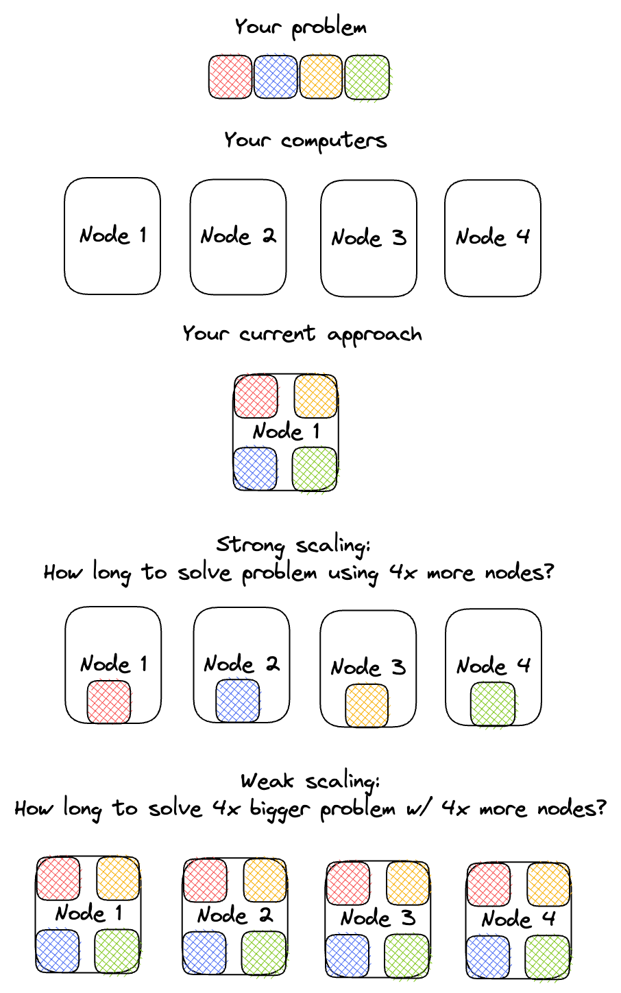
Strong vs. Weak Scaling Visual Explanation — This image illustrates the fundamental difference between strong and weak scaling. In **strong scaling**, the total problem size (4 colored squares) is fixed, and more resources (nodes) are added to solve it faster. In **weak scaling**, both the problem size and the number of resources are increased proportionally, with the goal of solving a larger problem in about the same amount of time.

Now let's dive into the formal definitions and implications of each.

Parallel Performance and Scalability – ACENET Summer School

The concepts of strong and weak scaling are central to analyzing parallel performance. This resource provides clear definitions, associating them with the laws we've learned and giving practical examples.

Read from the subsection 'Amdahl’s law' down to the end of 'Gustafson’s law'. Pay close attention to the descriptions and diagrams for 'Strong Scaling' and 'Weak Scaling', and the example problems given for each.

To synthesize and reinforce what you've just read, here is a summary table contrasting the two approaches:

Feature	Strong Scalability	Weak Scalability
Goal	Reduce time-to-solution for a fixed-size problem.	Solve a larger problem in a fixed amount of time.
Problem Size	Total size is constant.	Total size increases proportionally to processors $P$ .
Work per Processor	Decreases as $P$ increases.	Remains constant as $P$ increases.
Governing Law	Amdahl's Law (predicts an upper limit on speedup).	Gustafson's Law (predicts linear scaled speedup).
Primary Question	"How much faster can I solve my problem?"	"How much bigger of a problem can I solve?"
Typical Challenge	Diminishing returns as $P$ grows and overheads dominate.	Managing overhead that grows with $P$ (e.g., communication).

4. Putting It Into Practice: Scalability Studies

When you develop a parallel program, you typically perform a scalability study to characterize its performance. This involves running your code with an increasing number of processors and plotting the results.

Strong Scaling Study

Setup: Choose a representative, fixed problem size.
Execution: Run the program and measure the wall-clock time $T_{P}$ for $P = 1, 2, 4, 8, 16, \dots$ processors.
Analysis: Calculate speedup $S_{P} = T_{1} / T_{P}$ and efficiency $E_{P} = S_{P} / P$ for each $P$ .
Visualization: Plot $S_{P}$ vs. $P$ (ideally, a straight line) and $E_{P}$ vs. $P$ (ideally, a flat line at 1.0). In practice, the speedup curve will flatten, and the efficiency curve will droop downwards as Amdahl's law takes effect.

Weak Scaling Study

Setup: Choose a base problem size for a single processor. The key is to define how the problem grows with $P$ . For example, for a matrix operation on an $N \times N$ matrix, the work is proportional to $N^{2}$ . To keep work-per-processor constant, you would run on an $P N \times P N$ matrix with $P$ processors.
Execution: Run the program on the scaled problem size for $P = 1, 2, 4, 8, 16, \dots$ and measure the time $T_{P}$ . Let $T_{1}$ be the time for the base case on one processor.
Analysis: The main goal is to see if the execution time $T_{P}$ remains constant. Efficiency is calculated as $E_{P} = T_{1} / T_{P}$ .
Visualization: Plot $T_{P}$ vs. $P$ (ideally, a flat horizontal line) and $E_{P}$ vs. $P$ (ideally, a flat line at 1.0). A drop in efficiency indicates that parallel overhead is growing faster than the problem size.

These studies are crucial for understanding the performance characteristics of your code and identifying the point at which adding more processors is no longer beneficial.

Conclusion

In this lesson, we established a framework for measuring and analyzing the performance of parallel applications. You now have the tools to move beyond theoretical speedup and evaluate real-world scalability.

Key Takeaways:

Parallel Efficiency ( $E_{P} = S_{P} / P$ ) measures how effectively a parallel program uses available processors, quantifying the loss due to overhead.
Strong Scalability Analysis assesses performance on a fixed-size problem. It's governed by Amdahl's Law, and efficiency typically decreases as processors are added.
Weak Scalability Analysis assesses performance on a problem whose size scales with the number of processors. It's related to Gustafson's Law, and the goal is to maintain constant efficiency.
The choice between analyzing strong or weak scaling depends on whether your priority is to reduce execution time or increase problem complexity.

Preview of the Next Lesson

We've seen that efficiency is often limited by parallel overhead. A major source of this overhead, and a key factor in achieving good scalability, is how data is divided and distributed among processors. In our next lesson, we will explore common data distribution strategies for parallel processing: block, cyclic, and block-cyclic, and discuss how they affect performance and load balance.

Recommended resources