Parallel Prefix Sum (Scan) Algorithm Design in the PRAM Model

1. The Prefix Sum Problem and its Sequential Bottleneck

The prefix sum, or scan, operation takes an array of numbers and transforms it into an array where each element is the sum of all preceding elements in the original array (inclusive).

Given an input array X = [x₁, x₂, ..., xₙ], the inclusive prefix sum is an output array S = [s₁, s₂, ..., sₙ] where:
$s_i={\sum }_{j=1}^i{x}_j$
For example, the prefix sum of [3, 1, 4, 1, 5, 9] is [3, 4, 8, 9, 14, 23].

The sequential algorithm is simple:

s₁ = x₁
for i from 2 to n:
  sᵢ = sᵢ₋₁ + xᵢ

This algorithm clearly takes O(n) time. However, notice the critical data dependency: the calculation of sᵢ depends directly on the result of the previous calculation, sᵢ₋₁. This makes it impossible to parallelize this loop directly. Each step must wait for the one before it to complete. To create a parallel algorithm, we need a completely different approach.

The following short video segment explains this dependency and sets the stage for a parallel design.

2. A First Parallel Approach: The Hillis-Steele Algorithm

To break the sequential dependency, we need a way for elements to accumulate sums from their neighbors without waiting in a long chain. A classic approach is to have each element gather information from other elements at exponentially increasing distances. This is known as the Hillis-Steele algorithm.

The core idea is:

• In step 1, each element xᵢ adds the value from its left neighbor, xᵢ₋₁.
• In step 2, each element xᵢ adds the value from the element 2 positions to its left, xᵢ₋₂.
• In step k, each element xᵢ adds the value from the element 2ᵏ⁻¹ positions to its left.

We repeat this for log₂(n) steps. After log₂(n) steps, each element will have accumulated the sum of all elements to its left.

The following video provides a clear, animated visualization of this process.

Analysis of the Hillis-Steele Algorithm

Let's analyze this algorithm in the PRAM model:

• Parallel Time (Depth): The algorithm consists of log n stages. Each stage is a parallel for loop where n processors can perform an addition simultaneously. Each stage takes O(1) time. Therefore, the total parallel time is O(log n).
• Work: In each of the log n stages, we perform approximately n additions. The total number of operations is therefore n * log n. The work complexity is O(n log n).

Since the best sequential algorithm has a time complexity of O(n), this parallel algorithm is not work-efficient. It performs log n times more work. While it offers good speedup, the extra work can be a significant cost. Can we do better?

3. A Work-Efficient Design: The Blelloch Scan Algorithm

Yes, we can design an algorithm that achieves O(log n) time and is also work-efficient, with O(n) total work. A classic work-efficient algorithm is the Blelloch scan, which uses a divide-and-conquer approach that should feel familiar from your background in algorithms.

The algorithm can be described recursively and consists of two passes: an up-sweep (reduction) pass and a down-sweep (prefix construction) pass.

1. Up-Sweep Pass:

   • We pair up adjacent elements (x₂ᵢ₋₁, x₂ᵢ) and compute their sums in parallel. This halves the size of the array.
   • We then recursively call the algorithm on this new, smaller array of sums.
   • This process continues until we have a single element. This phase effectively builds a binary tree of partial sums from the bottom up.

2. Down-Sweep Pass:

   • We start from the root of the "imaginary" tree we built. The last element of the prefix sum is the total sum from the up-sweep (or 0 for an exclusive scan).
   • We traverse down the tree. At each level, we use the prefix sum passed down from the parent to calculate the correct prefix sums for its two children.
     • The right child's prefix sum is the value passed down from the parent plus the partial sum of the left child (computed during the up-sweep).
     • The left child's prefix sum is simply the value passed down from the parent.

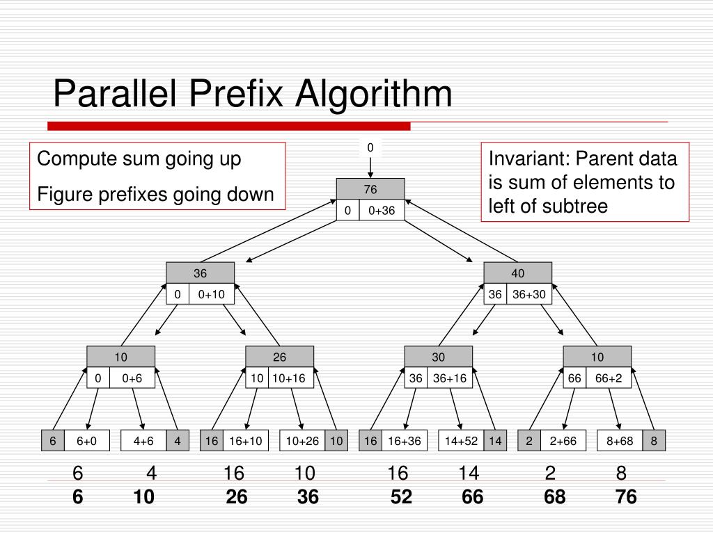
The following document provides a formal pseudocode for this recursive algorithm and analyzes its complexity.

Analysis of the Blelloch Scan Algorithm

As the document explains, the complexity can be described by recurrence relations:

• Time/Depth S(n): Each recursive step does O(1) parallel work before and after the recursive call on an input of half the size.
  $S(n)=S(n/2)+O(1)⟹S(n)=O(\log n)$
• Work W(n): Each step performs O(n) work (pairing up elements) before the recursive call on an n/2 sized problem.
  $W(n)=W(n/2)+O(n)⟹W(n)=O(n)$

This algorithm is therefore work-efficient and achieves the same O(log n) parallel time as the Hillis-Steele algorithm. It can be implemented on an EREW PRAM, making it theoretically very efficient.

4. Application: Parallel Array Compaction

Why is prefix sum so important? Because it lets us solve problems that seem inherently sequential. A great example is array compaction (or filtering).

Problem: Given an array A and a boolean flag array F, create a new array B that contains only the elements A[i] for which F[i] is true.

A sequential solution would iterate through the array with a counter for the output array index. This counter creates a data dependency.

With prefix sum, we can do this in parallel:

1. Convert the boolean array F to an integer array of 0s and 1s.
2. Perform a prefix sum on this new integer array. Let's call the result P.
3. The value P[i] now tells you the final destination index for the element A[i] in the output array B. Specifically, B[P[i] - 1] = A[i].
4. This final copy operation can be done in a single parallel step with n processors, as there are no data dependencies.

The bottleneck of the entire operation is the prefix sum itself.

Conclusion

In this lesson, we explored the design of parallel algorithms for the prefix sum problem within the PRAM model, a cornerstone of theoretical parallel computing.

Key Takeaways:

• The prefix sum (scan) operation has an inherent data dependency in its simple sequential form, requiring a different algorithmic structure for parallelization.
• The Hillis-Steele algorithm provides a simple, O(log n) time parallel solution but is not work-efficient, with O(n log n) work.
• The Blelloch scan algorithm, a two-pass divide-and-conquer approach, is a work-efficient parallel algorithm with O(n) work and O(log n) depth. This makes it asymptotically optimal.
• Prefix sum is a powerful primitive that enables the parallelization of many other problems, such as array compaction, by resolving data dependencies.

Preview of the Next Lesson

This lesson concludes our module on the theoretical principles of parallel algorithm analysis. We have built a solid foundation with concepts like data distribution, the PRAM model, and the design of key algorithms like reduction and prefix sum.

In the next module, we will transition from theory to practice. We'll begin exploring Shared-Memory Parallelism with OpenMP. Our first topic will be race conditions—a critical and common bug in parallel programs—and the synchronization mechanisms needed to prevent them. You'll see how the abstract ideas of parallel operations and data dependencies manifest in real C++ code.