Density Matrix and Trace Formalism

Introduction

In our last lesson, we explored how to describe composite quantum systems using the tensor product, which led us to the uniquely quantum phenomenon of entanglement. We saw that in an entangled pure state, like $∣Ψ ⟩_{A B}$ , the system as a whole is in a definite state, but the individual subsystems A and B are not. This raises a critical question: if a state vector is insufficient, what mathematical object can describe the state of a subsystem like A?

This lesson introduces the density operator, or density matrix, which provides a complete and universal description for any quantum state, whether it's a pure state described by a state vector, a subsystem of a larger entangled system, or a statistical ensemble where our knowledge is incomplete. You will learn how to construct the density matrix $ρ$ for both pure and mixed states, and how to use the powerful trace formalism to compute expectation values and measurement probabilities. This tool is fundamental not only for understanding entanglement and open quantum systems but also for foundational topics like quantum statistical mechanics.

From Subsystems to Density Matrices

The most compelling motivation for the density matrix arises directly from our previous discussion on entanglement. Let's consider a bipartite system AB in a pure state $∣Ψ ⟩_{A B}$ , but an observer, Alice, has access only to subsystem A. What can she say about her system's state?

If Alice measures an observable $M^_{A}$ (which acts as $M^_{A} \otimes I_{B}$ on the full space), the expectation value is $⟨ Ψ_{A B} ∣ M^_{A} \otimes I_{B} ∣ Ψ_{A B} ⟩$ . It turns out that unless $∣Ψ ⟩_{A B}$ is a simple product state, this expectation value cannot be written as $⟨ ψ_{A} ∣ M^_{A} ∣ ψ_{A} ⟩$ for any single state vector $∣ ψ_{A} ⟩$ . A new formalism is needed.

The following lecture by Professor John Preskill provides an excellent derivation of how the description of a subsystem naturally leads to the density operator.

Ph CS 219A Lecture 2 Density Operator

This video, "Ph CS 219A Lecture 2 Density Operator," derives the density operator from first principles by considering a subsystem of a larger quantum system.

First, watch the initial derivation for a simple case. Prof. Preskill considers a specific entangled state and shows that the expectation value of an observable on Alice's side can be elegantly expressed using a new operator, \rho_A, and the trace. Next, watch the general derivation. This extends the argument to an arbitrary bipartite state and formally introduces the partial trace as the operation used to "trace out" or ignore Bob's system, yielding Alice's reduced density matrix: \rho_A = \text{Tr}_B(\rho_{AB}).

As you saw in the video, the state of subsystem A is completely characterized by its reduced density matrix, $ρ_{A}$ , obtained by performing a partial trace over subsystem B:

ρ_{A} = Tr_{B} (∣Ψ ⟩_{A B} ⟨ Ψ ∣_{A B})

The partial trace is the quantum analogue of marginalizing a joint probability distribution in classical probability theory. It gives us a valid statistical description of a subsystem by averaging over the degrees of freedom we cannot access.

The General Density Operator: Pure and Mixed States

The formalism we just developed for subsystems is powerful enough to describe any quantum state. We can now define the two fundamental types of states in this language.

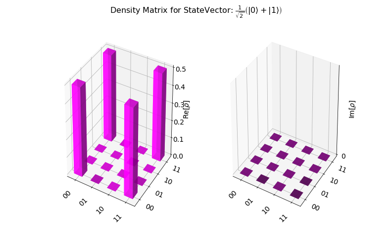
Pure States: A system is in a pure state if its state is described by a single state vector $∣ ψ ⟩$ . The corresponding density operator is simply the projection operator onto that state: $ρ_{pure} = ∣ ψ ⟩ ⟨ ψ ∣$ The state $(∣0 ⟩ + ∣1 ⟩) / 2$ is a pure state. Its density matrix $ρ$ would have four equal real components, as visualized below.

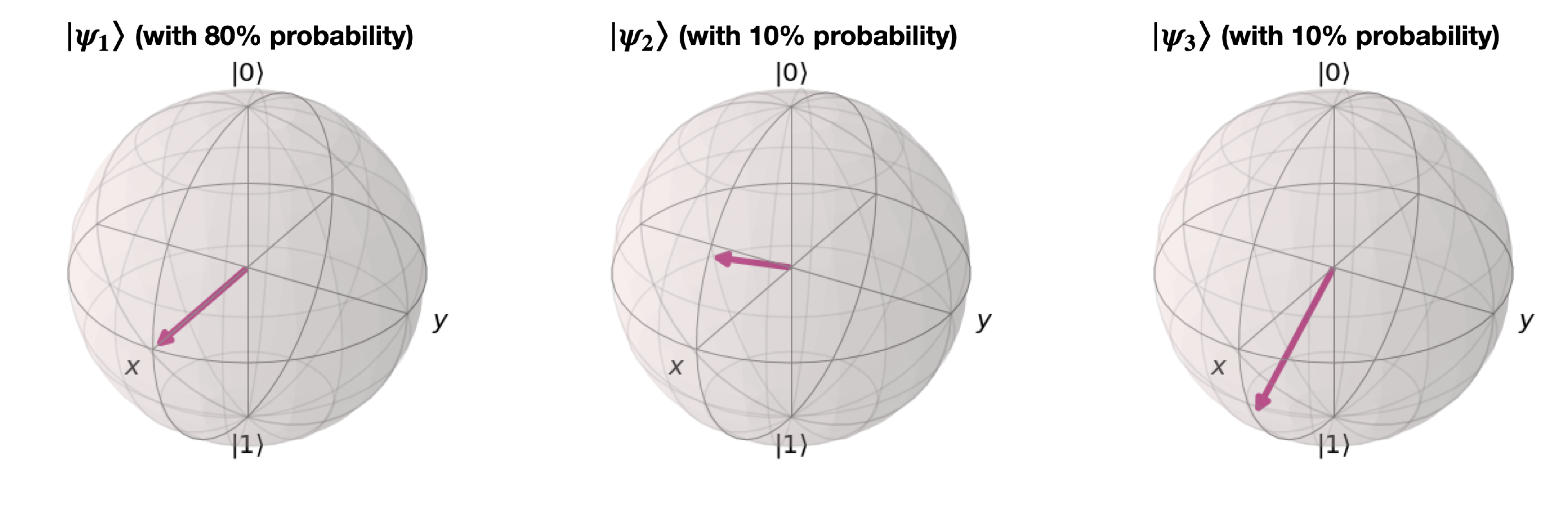
A 3D bar chart showing the real and imaginary parts of the density matrix for the pure state $(|0\rangle + |1\rangle)/\sqrt{2}$. The real part has four equal entries of 0.5, and the imaginary part is zero.

Mixed States: A system is in a mixed state if it is a statistical ensemble of pure states. This means the system is in state $∣ ψ_{k} ⟩$ with a classical probability $p_{k}$ , where $\sum_{k} p_{k} = 1$ . This uncertainty is not the inherent probabilistic nature of quantum measurement, but rather a classical lack of knowledge about the system's preparation. A subsystem of an entangled pure state is a canonical example of a mixed state.

The density operator for a mixed state is the weighted average of the pure state density operators in the ensemble:
$ρ_{mixed} = k \sum p_{k} ∣ ψ_{k} ⟩ ⟨ ψ_{k} ∣ = k \sum p_{k} ρ_{k}$
This is a convex combination of pure-state projectors. It's crucial to realize that different statistical mixtures can result in the same density matrix. The density matrix contains all physically accessible information; the underlying ensemble composition is not unique and not directly measurable.

An illustration of the concept behind a mixed state. The system has an 80% chance of being in state $|\psi_1\rangle$, a 10% chance of being in $|\psi_2\rangle$, and a 10% chance of being in $|\psi_3\rangle$. The resulting density matrix would be $\rho = 0.8|\psi_1\rangle\langle\psi_1| + 0.1|\psi_2\rangle\langle\psi_2| + 0.1|\psi_3\rangle\langle\psi_3|$.

The following reading provides several concrete examples, including the physically important case of a system in thermal equilibrium, which will be familiar from your studies in statistical mechanics.

Entanglement, Density Matrices, and Decoherence

This excerpt from MIT OpenCourseWare notes provides several clear and important examples of density matrices.

Read section 2.2 Examples. Pay attention to how the density matrix is constructed for: A general pure state. A spin-1/2 state, connecting to the Bloch sphere representation. Note the important result that for a singlet state, Bob's reduced density matrix is the maximally mixed state, independent of Alice's measurement basis. The maximally mixed state, \rho = \mathbb{I}/d. The thermal (Gibbs) state, \rho = e^{-\beta H} / Z, which is a cornerstone of quantum statistical mechanics.

Properties and the Trace Formalism

For an operator $ρ$ to be a valid density matrix, it must satisfy three fundamental properties. These properties ensure that $ρ$ can represent a physical state and that any predictions derived from it are sensible.

A $d \times d$ matrix $ρ$ is a valid density operator if and only if:

It has unit trace: $Tr (ρ) = 1$ . This is the statement of probability conservation.
It is Hermitian: $ρ^{†} = ρ$ . This ensures that its eigenvalues are real, which we will see correspond to probabilities.
It is positive semi-definite: $ρ \geq 0$ . This means that for any vector $∣ ϕ ⟩$ , the expectation value $⟨ ϕ ∣ ρ ∣ ϕ ⟩ \geq 0$ . This guarantees that all its eigenvalues are non-negative.

The following resources formalize these conditions and show how to use $ρ$ to compute physical quantities.

Entanglement, Density Matrices, and Decoherence

This reading formally establishes the rules for density operators and their use in measurements.

First, read Section 3 The general rule for density operators and its subsections. This section rigorously proves that the three conditions (unit trace, Hermiticity, and positive semi-definiteness) are necessary and sufficient for an operator to be a valid density matrix. Next, read Section 4.2 Measurement. This part derives the central formulas for calculating measurement probabilities using the density matrix: P_j = \langle v_j | \rho | v_j \rangle = \text{Tr}(\rho |v_j\rangle\langle v_j|).

With the density matrix defined, the calculation of all observable properties of a system is unified under the trace operation.

Expectation Value: The expectation value of an observable $A^$ in the state $ρ$ is given by: $⟨ A^⟩ = Tr (ρ A^)$
Measurement Probability: The probability of obtaining the outcome $a_{n}$ when measuring $A^$ is: $P (a_{n}) = Tr (ρ P_{n})$ where $P_{n}$ is the projection operator onto the eigenspace corresponding to the eigenvalue $a_{n}$ .

These two rules are among the most important and practical formulas in all of quantum mechanics.

Distinguishing Pure and Mixed States

Since the same formalism applies to both pure and mixed states, how can we tell them apart just by looking at $ρ$ ? The key lies in a quantity called the purity, defined as $Tr (ρ^{2})$ .

For a pure state, $ρ = ∣ ψ ⟩ ⟨ ψ ∣$ . Since it's a projector, it is idempotent: $ρ^{2} = ρ$ . Therefore, its purity is: $Tr (ρ^{2}) = Tr (ρ) = 1$
For a mixed state, $ρ = \sum_{k} p_{k} ρ_{k}$ , where at least two $p_{k} > 0$ . It can be shown that $ρ$ is not idempotent. Let the eigenvalues of $ρ$ be ${λ_{i}}$ . Since $ρ$ is a valid density matrix, we know $λ_{i} \geq 0$ and $\sum_{i} λ_{i} = 1$ . The purity is $Tr (ρ^{2}) = \sum_{i} λ_{i}^{2}$ . Because $λ_{i} \leq 1$ , we have $λ_{i}^{2} \leq λ_{i}$ , with equality holding only if $λ_{i}$ is 0 or 1. For a mixed state, at least two eigenvalues must be non-zero and less than 1, which leads to the strict inequality: $Tr (ρ^{2}) = i \sum λ_{i}^{2} < i \sum λ_{i} = 1$

Thus, we have a simple and definitive criterion:

$Tr (ρ^{2}) = 1 ⟺ ρ$ is a pure state.
$Tr (ρ^{2}) < 1 ⟺ ρ$ is a mixed state.

The following video provides an exceptionally clear walkthrough of this crucial distinction.

Density operator for mixed quantum states

The video "Density operator for mixed quantum states" gives a concise explanation of how to differentiate pure and mixed states.

Please watch the section on this topic. The presenter clearly derives the idempotency property for pure states and shows why \text{Tr}(\rho^2) < 1 for mixed states.

Conclusion

This lesson has introduced the density operator as the ultimate tool for describing quantum states. It elegantly handles situations involving classical uncertainty (statistical ensembles) and purely quantum phenomena, such as describing subsystems of entangled states. By completing the mathematical formalism of quantum mechanics, we are now fully equipped to state the theory's foundations.

Key Takeaways:

The density operator $ρ$ provides a complete description of any quantum state.
For a pure state $∣ ψ ⟩$ , $ρ = ∣ ψ ⟩ ⟨ ψ ∣$ . For a mixed state (ensemble ${p_{k}, ∣ ψ_{k} ⟩}$ ), $ρ = \sum_{k} p_{k} ∣ ψ_{k} ⟩ ⟨ ψ_{k} ∣$ .
A subsystem A of a larger system AB is described by the reduced density matrix $ρ_{A} = Tr_{B} (ρ_{A B})$ .
Any valid density matrix must be Hermitian ( $ρ^{†} = ρ$ ), have unit trace ( $Tr (ρ) = 1$ ), and be positive semi-definite ( $ρ \geq 0$ ).
Expectation values and measurement probabilities are computed using the trace formalism: $⟨ A ⟩ = Tr (ρ A)$ and $P (a_{n}) = Tr (ρ P_{n})$ .
The purity, $Tr (ρ^{2})$ , serves as a definitive test: it is 1 for a pure state and less than 1 for a mixed state.

With this, we conclude our exploration of the mathematical formalism. In the next module, we will begin our study of the Postulates of Quantum Mechanics. The first lesson will assemble all the concepts we've developed—Hilbert spaces, operators, tensor products, and density matrices—into a single, cohesive axiomatic framework that forms the bedrock of the theory.

Recommended resources