Time-Energy Uncertainty: Derivation and Interpretation

Introduction

In our last lesson, we explored the Schrödinger, Heisenberg, and Interaction pictures, establishing that the description of time evolution in quantum mechanics is not unique. A critical point that emerged was the special role of time: in all these standard formulations, $t$ is a classical parameter, not a quantum observable represented by a Hermitian operator. This observation is the perfect entry point for today's topic.

We will now derive the celebrated time-energy uncertainty relation, $Δ E Δ t \geq ℏ/2$ . Your primary goal for this lesson is not just to follow the derivation but to deeply understand why this relation is conceptually distinct from its more famous counterpart, the position-momentum uncertainty principle. We will unravel the precise meaning of the quantity $Δ t$ and see how it quantifies the dynamics of a system, rather than an uncertainty in a measurement of time itself.

Let's begin by watching a short video that clearly frames the central issue.

The time-energy uncertainty principle

This video from the channel "Professor M does Science" immediately highlights the core distinction: time is a parameter, not an observable.

Watch the introductory segment from the beginning. It sets the stage by contrasting the time-energy relation with the position-momentum relation, which involves two observables.

The Problem with a Time Operator

The generalized uncertainty principle, which we derived for two arbitrary observables $A$ and $B$ ,

(Δ A)^{2} (Δ B)^{2} \geq \frac{1}{2 i} ⟨[A, B]⟩^{2}

is the foundation for the position-momentum relation, $Δ x Δ p \geq ℏ/2$ , because the commutator $[x, p] = i ℏ$ is a non-zero constant.

It is natural to wonder if we can do the same for energy and time. Could we define a "time operator" $T$ that is canonically conjugate to the Hamiltonian $H$ , satisfying $[H, T] = i ℏ$ ? If such an operator existed, the time-energy uncertainty relation would follow trivially. However, a profound theorem stands in the way.

For physically realistic systems, such an operator cannot exist. The reasoning is subtle and provides a deep insight into the structure of quantum mechanics. The following text by John Baez offers an excellent and accessible explanation.

The Time-Energy Uncertainty Relation - UCR Math

This article clearly explains the theoretical obstacle to defining a time operator.

Read the section beginning with "Hey, that's way cool!". The key argument relies on the Stone-von Neumann theorem and the fact that physical Hamiltonians must be bounded below (i.e., have a ground state).

As you've just read, the requirement for a physical system to have a lowest energy state (to be stable) is fundamentally incompatible with the existence of a time operator that is canonically conjugate to its Hamiltonian. This forces us to seek a different, more nuanced path to the time-energy uncertainty relation.

The Mandelstam-Tamm Formulation

The rigorous derivation, first formulated by Leonid Mandelstam and Igor Tamm, cleverly bypasses the need for a time operator. The strategy is to start with the generalized uncertainty principle, but apply it to the Hamiltonian $H$ and an arbitrary observable $Q$ that does not explicitly depend on time. The "time" aspect then emerges not from an operator, but from the dynamics of the observable $Q$ .

Let's walk through this elegant derivation. The following video provides a concise and animated guide.

The time-energy uncertainty principle

This video continues by setting up the problem with two observables, H and A (our Q), and then uses the Ehrenfest theorem to connect their commutator to the time evolution of the system.

Please watch the main derivation, starting from the setup. The key steps are: Writing down the generalized uncertainty principle for H and an observable A. Using the result \frac{d\langle A \rangle}{dt} = \frac{1}{i\hbar} \langle [H, A] \rangle to relate the commutator to the rate of change of \langle A \rangle. Substituting this back into the uncertainty inequality. Defining the characteristic time \Delta t and energy uncertainty \Delta E.

Let's summarize the key mathematical steps you just saw.

We begin with the standard uncertainty relation between the Hamiltonian $H$ and some time-independent observable $Q$ : $Δ H Δ Q \geq \frac{1}{2} ∣ ⟨[H, Q]⟩ ∣$
We then use the equation for the time evolution of the expectation value of $Q$ (which you may recognize as a specific case of the Heisenberg equation of motion): $\frac{d ⟨ Q ⟩}{d t} = \frac{1}{i ℏ} ⟨[H, Q]⟩ ⟹ ∣ ⟨[H, Q]⟩ ∣ = ℏ \frac{d ⟨ Q ⟩}{d t}$
Substituting this into the inequality yields: $Δ H Δ Q \geq \frac{ℏ}{2} \frac{d ⟨ Q ⟩}{d t}$
This is a precise inequality. To arrive at the familiar form, we simply rearrange and define a quantity $Δ t_{Q}$ which has units of time: $Δ t_{Q} \equiv \frac{Δ Q}{∣ d ⟨ Q ⟩ / d t ∣}$
With this definition, and setting $Δ E \equiv Δ H$ , we arrive at the Mandelstam-Tamm uncertainty relation: $Δ E Δ t_{Q} \geq \frac{ℏ}{2}$

Interpretation: A Tale of Two Uncertainties

The crucial part of this lesson is understanding what $Δ t_{Q}$ actually represents. Unlike $Δ x$ , which is the statistical spread in outcomes of position measurements, $Δ t_{Q}$ is not an uncertainty in a measurement of time.

Instead, $Δ t_{Q}$ is the characteristic time scale for the evolution of the system. It represents the amount of time it takes for the expectation value of the observable $Q$ to change by one standard deviation. It answers the question: "How long must I wait to see a significant change in the system, as measured by the observable Q?"

The following segment of the video provides an excellent visual explanation of this interpretation.

The time-energy uncertainty principle

This final part of the video contrasts the time-energy relation with the position-momentum relation and uses animated distributions to explain the meaning of Δt.

Watch from this point to the end. Pay close attention to the conceptual distinction and the example of a stationary state.

As the video explained, the time-energy uncertainty principle connects the energy spread of a state to its rate of evolution.

A state with a very small energy uncertainty $Δ E$ must be a superposition of only a few energy eigenstates that are very close in energy. Consequently, it evolves very slowly, leading to a large $Δ t_{Q}$ .
In the limit where a state is a single energy eigenstate, $Δ E = 0$ . This is a stationary state. For such a state, $d ⟨ Q ⟩ / d t = 0$ for all $Q$ , meaning $Δ t_{Q}$ is infinite. The state never changes, which is perfectly consistent with the uncertainty relation.
Conversely, a state that evolves very rapidly (small $Δ t_{Q}$ ) must be a superposition of many, widely spaced energy eigenstates, and thus will have a large energy uncertainty $Δ E$ .

Application: Lifetime and Decay Width

A very common and intuitive application of this principle is in the context of unstable particles or excited states. Consider an excited atomic state that decays to the ground state by emitting a photon. This state has a finite lifetime, $τ$ .

This lifetime $τ$ is precisely the characteristic timescale over which the system undergoes a significant change (i.e., it decays). We can therefore associate $τ$ with $Δ t$ . The uncertainty principle then implies that the energy of this unstable state cannot be perfectly sharp. It must have an intrinsic energy uncertainty, or "decay width," $Γ$ , such that:

Γ \cdot τ ≳ \frac{ℏ}{2}

States with very short lifetimes are broad in energy, while very long-lived (metastable) states are extremely sharp. This is a direct, measurable consequence of the time-energy uncertainty principle. The energy distribution of such a short-lived state is often described by a Lorentzian profile, also known as a Breit-Wigner distribution in high-energy physics.

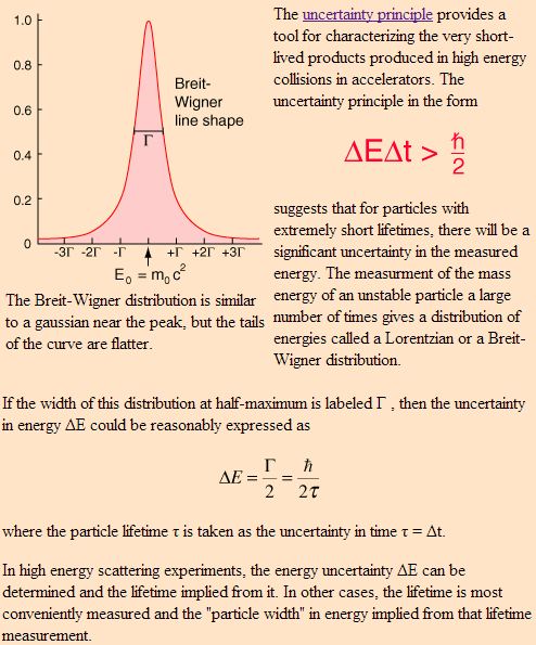
This image illustrates the connection between the lifetime of an unstable particle and its energy distribution. The width of the energy distribution at half its maximum value, denoted by $\Gamma$, is inversely proportional to the particle's lifetime $\tau$. This "particle width" is a direct manifestation of the time-energy uncertainty principle.

Given your work in spectroscopy and condensed matter, you have likely encountered the concept of lifetime broadening of spectral lines. This phenomenon is a direct physical manifestation of the time-energy uncertainty principle.

Conclusion

Today we have dissected one of the most frequently cited, yet often misinterpreted, principles in quantum mechanics. By grappling with the non-existence of a time operator, we arrived at a more profound understanding of the relationship between energy and time.

Key Takeaways:

The time-energy uncertainty relation is conceptually different from the position-momentum relation because time is a parameter, not an observable represented by a Hermitian operator in standard quantum mechanics. A self-adjoint time operator conjugate to a Hamiltonian with a lower-bounded spectrum cannot exist.
The quantity $Δ t$ in the relation $Δ E Δ t \geq ℏ/2$ is not an uncertainty in a time measurement. It is the characteristic timescale for the system to evolve significantly, defined as $Δ t_{Q} = Δ Q /∣ d ⟨ Q ⟩ / d t ∣$ for some observable $Q$ .
The principle states that systems with a narrow spread of energy ( $Δ E$ ) evolve slowly (large $Δ t$ ), while rapidly evolving systems (small $Δ t$ ) must have a large energy spread.
A practical application is the relationship between the lifetime $τ$ of an unstable state and its energy width $Γ$ , often expressed as $Γ τ \approx ℏ$ .

In our next lesson, we will construct a Gaussian wave packet for a free particle. This will serve as a concrete mathematical example of a non-stationary state, allowing us to explicitly observe its time evolution, the spreading of the wave packet, and how both the position-momentum and time-energy uncertainty principles manifest in its dynamics.

Recommended resources

Introduction

The Problem with a Time Operator

The Mandelstam-Tamm Formulation

Interpretation: A Tale of Two Uncertainties

Application: Lifetime and Decay Width

Conclusion